class: center, middle, inverse, title-slide # Decision Trees ## An introduction ### Daniel Anderson ### Week 7, Class 1 --- # Agenda * Overview of CART models * Finding an optimal tree - complexity parameter * Feature interpretation (quickly) --- # Overview * Non-parametric (do not make any distributional assumptions) * Use splitting rules to divide features into non-overlapping regions, where the cases within each region are similar * Basically the stepping stone for more complex models - generally don't work great on their own. --- # Classification * Decision trees are often easiest to think of, initially, through a classification problem * Think about the titanic dataset - did passengers aboard survive? --- # An example from the titanic  --- # Some terminology 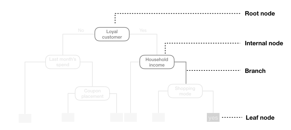 Note the leaf node is also called the terminal node --- # Splitting rules * .b[C]lassification .b[a]nd .b[r]egression .b[t]rees (CART) - Partition training data into homogeneous subgroups through recursive splitting (yes/no) until some criterion is reached - Recursive because each split depends on prior splits -- * At each node, find the "best" partition - search all possible splits on all possible variables -- * How to define best? - Regression + SSE: `\(\Sigma_{R1}(y_i - c_1)^2 + \Sigma_{R2}(y_i - c_2)^2\)` * `\(c\)` is the prediction (mean of cases in the region), which starts as a constant and is updated * `\(R\)` is the region - Classification + Cross-entropy or Gini impurity (default) --- # Gini impurity * [Gini impurity](https://en.wikipedia.org/wiki/Decision_tree_learning#Gini_impurity) is not the same thing as the [Gini coefficient](https://en.wikipedia.org/wiki/Gini_coefficient) (this was very confusing for me) * Default measure of lack of fit used by `rpart`. -- For a two class situation: $$ D_i = 1 - P(c_1)^2 - P(c_2)^2 $$ where `\(P(c_1)\)` and `\(P(c_2)\)` are the probabilities of being in Class 1 or 2, respectively, for node `\(i\)` --- For a multi-class solution $$ D_i = 1 - \Sigma(p_i)^2 $$ In either case: * When `\(D = 0\)`, the node is "pure" (perfect classification) * When `\(D = 0.5\)`, the node is random (flip a coin) --- # A couple examples * Say your terminal node has 75% in one class, for a binary decision. The Gini index would be .left[ $$ `\begin{aligned} D &= 1 - (0.75^2 + 0.25^2) \\\ D &= 1 - (0.5625 + 0.0625) \\\ D &= 1 - 0.625 \\\ D &= 0.375 \end{aligned}` $$ ] --- # 90% $$ `\begin{aligned} D &= 1 - (0.90^2 + 0.10^2) \\ D &= 1 - (0.81 + 0.01) \\ D &= 1 - 0.82 \\ D &= 0.18 \end{aligned}` $$ -- ### Take home message - lower values mean better classifications --- background-image: url(https://bradleyboehmke.github.io/HOML/07-decision-trees_files/figure-html/decision-stump-1.png) background-size:cover # Visualizing splits --- background-image: url(https://bradleyboehmke.github.io/HOML/07-decision-trees_files/figure-html/decision-stump-2.png) background-size:cover --- # Replicating the book ### Generate some data ```r set.seed(42) n <- 200 # number of data points x <- seq(0, 3.5, length.out = n) a <- 5 b <- 2 error <- rnorm(n) amp <- 4 # generate data and calculate "y" y <- a*sin(b*x)+error*amp ``` --- ```r library(tidyverse) sin_df <- tibble(x = x, y = y, truth = a*sin(b*x)) ggplot(sin_df, aes(x, y)) + geom_point() + geom_line(aes(y = truth)) ``` <!-- --> --- # Fit a simple model - one split ```r library(rpart) library(rpart.plot) mean(sin_df$y) ``` ``` ## [1] 0.0731617 ``` ```r stump <- rpart(y ~ x, data = sin_df, * control = list(maxdepth = 1)) # limit tree depth ``` --- ```r summary(stump) ``` ``` ## Call: ## rpart(formula = y ~ x, data = sin_df, control = list(maxdepth = 1)) ## n= 200 ## ## CP nsplit rel error xerror xstd ## 1 0.3269998 0 1.0000000 1.0163112 0.07897900 ## 2 0.0100000 1 0.6730002 0.7084092 0.06699837 ## ## Variable importance ## x ## 100 ## ## Node number 1: 200 observations, complexity param=0.3269998 ## mean=0.0731617, MSE=28.39826 ## left son=2 (106 obs) right son=3 (94 obs) ## Primary splits: ## x < 1.644472 to the right, improve=0.3269998, (0 missing) ## ## Node number 2: 106 observations ## mean=-2.796499, MSE=20.74408 ## ## Node number 3: 94 observations ## mean=3.309162, MSE=17.27164 ``` --- # View the tree ```r rpart.plot(stump) ``` <!-- --> --- # Visualize the split ```r sin_df %>% mutate(pred = predict(stump)) %>% ggplot(aes(x, y)) + geom_point() + geom_line(aes(y = truth)) + geom_line(aes(y = pred), color = "red") ``` <!-- --> --- # More complicated * Note that we only have one predictor - but we can use that predictor multiple times * Let's specify it again with two splits ```r twosplit <- rpart(y ~ x, data = sin_df, control = list(maxdepth = 2)) ``` --- # View tree ```r rpart.plot(twosplit) ``` <!-- --> --- # Visualize two splits ```r sin_df %>% mutate(pred = predict(twosplit)) %>% ggplot(aes(x, y)) + geom_point() + geom_line(aes(y = truth)) + geom_line(aes(y = pred), color = "red") ``` <!-- --> --- # More complicated Let's try with 10 splits ```r tensplit <- rpart(y ~ x, data = sin_df, control = list(minsplit = 0, cp = 0, maxdepth = 10)) ``` Notice I've changed the complexity parameter, `cp`, to be 0, which will force it to grow a full tree (more on this in a bit) --- ```r rpart.plot(tensplit) ``` <!-- --> --- ```r sin_df %>% mutate(pred = predict(tensplit)) %>% ggplot(aes(x, y)) + geom_point() + geom_line(aes(y = truth)) + geom_line(aes(y = pred), color = "red") ``` <!-- --> --- # Tree depth * The above probably leaves you thinking... how deep should I grow the trees? + Super deep - likely to overfit (high variance) + Super shallow - likely to underfit (high bias) -- ### Two primary approaches * Stop the tree early * Grow the tree deep, then prune it back --- # Stopping early Two primary approaches: * Limit the depth * Limit the *n* size within a terminal node --- class: inverse background-image: url(https://bradleyboehmke.github.io/HOML/07-decision-trees_files/figure-html/dt-early-stopping-1.png) background-size:contain --- # Pruning * Tree is grown to a great depth, increasing the likelihood that important interactions in the data are captured. * The large tree is "pruned" to a smaller subtree that captures (ideally) only the meaningful variation in the data. -- ### Cost complexity * Typically denoted `\(\alpha\)`, the cost complexity introduces a penalization to the SSE (discussed earlier). $$ SSE + \alpha\mid{T}\mid $$ where `\(T\)` is the number of terminal nodes/leafs --- # Cost complexity * The equation on the previous slide is .red[minimized] and, for a given `\(\alpha\)`, we identify (from the large tree) a subtree with the lowest penalized error. * There is a clear association between this penalization and lasso regression. * `\(\alpha\)` is typically determined via grid search with cross-validation - smaller penalties = more complex trees - larger penalties = smaller trees * When pruning a tree, the reduction in the SSE must be larger than the cost complexity penalty. --- ## What about for classification problems? The basic structure is the same - split the predictor space into regions, make predictions based on the most prominent class Let's look at the [penguins](https://allisonhorst.github.io/palmerpenguins/) dataset. ```r library(palmerpenguins) head(penguins) ``` ``` ## # A tibble: 6 x 8 ## species island bill_length_mm bill_depth_mm flipper_length_mm body_mass_g ## <fct> <fct> <dbl> <dbl> <int> <int> ## 1 Adelie Torgersen 39.1 18.7 181 3750 ## 2 Adelie Torgersen 39.5 17.400 186 3800 ## 3 Adelie Torgersen 40.300 18 195 3250 ## 4 Adelie Torgersen NA NA NA NA ## 5 Adelie Torgersen 36.7 19.3 193 3450 ## 6 Adelie Torgersen 39.300 20.6 190 3650 ## # … with 2 more variables: sex <fct>, year <int> ``` --- Fit a model predicting the species. ```r class <- rpart(species ~ bill_length_mm + flipper_length_mm , data = penguins, method = "class") ``` Notice I've added `method = class` to specify it as a classification problem. If `y` is a factor it will do this automatically, but good to be specific. --- ```r rpart.plot(class) ``` <!-- --> --- <!-- --> --- # An applied example * Let's look at the Kaggle data science bowl data again ```r train <- read_csv( here::here("data", "data-science-bowl-2019", "train.csv"), n_max = 5e4 # Limit cases for speed of producing these slides ) %>% select(-event_data) train_labels <- read_csv( here::here("data", "data-science-bowl-2019", "train_labels.csv") ) ``` --- # Inspect the keys ```r train_labels %>% count(game_session, installation_id) %>% filter(n > 1) ``` ``` ## # A tibble: 0 x 3 ## # … with 3 variables: game_session <chr>, installation_id <chr>, n <int> ``` ```r train %>% count(game_session, installation_id) %>% filter(n > 1) ``` ``` ## # A tibble: 517 x 3 ## game_session installation_id n ## <chr> <chr> <int> ## 1 0132ad94d2c5e234 00e17272 90 ## 2 01a1a7d058854c47 00a803f0 19 ## 3 01d44d1b32c3da7f 00691033 56 ## 4 021462bb2394e97b 00691033 126 ## 5 02546c6aa91244cd 00cef781 90 ## 6 02d9c0f8b9d25cf8 00fa8681 24 ## 7 031f9b0a80aa39aa 00e536bf 83 ## 8 0334295374a6db00 00d8a6f2 125 ## 9 0336db4dee65ad4b 0006a69f 131 ## 10 034ed83ac5546c2f 00129856 52 ## # … with 507 more rows ``` --- # Join the data ```r k_train <- left_join(train, train_labels) # check join is as expected nrow(train); nrow(k_train) ``` ``` ## [1] 50000 ``` ``` ## [1] 50000 ``` --- # Select only vars in test data ```r model_set <- k_train %>% select(event_count, event_code, game_time, title, world, accuracy_group) %>% drop_na(accuracy_group) model_set ``` ``` ## # A tibble: 3,689 x 6 ## event_count event_code game_time title world ## <dbl> <dbl> <dbl> <chr> <chr> ## 1 1 2000 0 Mushroom Sorter (Assessment) TREETOPCITY ## 2 2 2025 37 Mushroom Sorter (Assessment) TREETOPCITY ## 3 3 3010 37 Mushroom Sorter (Assessment) TREETOPCITY ## 4 4 3110 3901 Mushroom Sorter (Assessment) TREETOPCITY ## 5 5 3010 3901 Mushroom Sorter (Assessment) TREETOPCITY ## 6 6 4025 6475 Mushroom Sorter (Assessment) TREETOPCITY ## 7 7 3110 6475 Mushroom Sorter (Assessment) TREETOPCITY ## 8 8 3021 6475 Mushroom Sorter (Assessment) TREETOPCITY ## 9 9 3121 7084 Mushroom Sorter (Assessment) TREETOPCITY ## 10 10 4025 8400 Mushroom Sorter (Assessment) TREETOPCITY ## # … with 3,679 more rows, and 1 more variable: accuracy_group <dbl> ``` --- # Splits Initial split, extract training data, create `\(k\)`-fold CV object. ```r library(tidymodels) splt <- initial_split(model_set) train <- training(splt) cv <- vfold_cv(train) ``` --- # Develop a simple recipe ```r rec <- recipe(accuracy_group ~ ., data = train) %>% step_mutate(accuracy_group = as.factor(accuracy_group)) rec ``` ``` ## Data Recipe ## ## Inputs: ## ## role #variables ## outcome 1 ## predictor 5 ## ## Operations: ## ## Variable mutation for accuracy_group ``` --- # Set model specification * set arbitrary cost complexity parameter and minimum n ```r mod_random1 <- decision_tree() %>% set_mode("classification") %>% set_engine("rpart") %>% set_args(cost_complexity = 0.01, min_n = 5) ``` --- # Fit the arbitrary model * Fit it to the full training set, just to get a feel for it ```r m01 <- fit(mod_random1, accuracy_group ~ ., prep(rec) %>% bake(train)) acc_check <- tibble( truth = prep(rec) %>% bake(train) %>% pull(accuracy_group), estimate = predict(m01$fit, type = "class") ) accuracy(acc_check, truth, estimate) ``` ``` ## # A tibble: 1 x 3 ## .metric .estimator .estimate ## <chr> <chr> <dbl> ## 1 accuracy multiclass 0.6566679 ``` --- # View the tree Five splits ```r rpart.plot(m01$fit) ``` <!-- --> --- # Try different hyperparameters ```r mod_random2 <- decision_tree() %>% set_mode("classification") %>% set_engine("rpart") %>% set_args(cost_complexity = 0, min_n = 2) m02 <- fit(mod_random2, accuracy_group ~ ., prep(rec) %>% bake(train)) acc_check <- tibble( truth = prep(rec) %>% bake(train) %>% pull(accuracy_group), estimate = predict(m02$fit, type = "class") ) accuracy(acc_check, truth, estimate) ``` ``` ## # A tibble: 1 x 3 ## .metric .estimator .estimate ## <chr> <chr> <dbl> ## 1 accuracy multiclass 0.9833755 ``` --- class:center middle # 😳  --- # Check these two models with CV ```r random1_cv <- fit_resamples(mod_random1, rec, cv) random2_cv <- fit_resamples(mod_random2, rec, cv) collect_metrics(random1_cv) ``` ``` ## # A tibble: 2 x 5 ## .metric .estimator mean n std_err ## <chr> <chr> <dbl> <int> <dbl> ## 1 accuracy multiclass 0.6566879 10 0.01103005 ## 2 roc_auc hand_till 0.7884877 10 0.008771908 ``` ```r collect_metrics(random2_cv) ``` ``` ## # A tibble: 2 x 5 ## .metric .estimator mean n std_err ## <chr> <chr> <dbl> <int> <dbl> ## 1 accuracy multiclass 0.6328258 10 0.009675918 ## 2 roc_auc hand_till 0.7184599 10 0.006283661 ``` ---  -- The second model is really overfit. In fact, it has .b[813] splits! --- # Tune hyperparameters * Three different hyperparameters: + `cost_complexity()`: This is `\(\alpha\)`, what rpart calls `Cp` + `tree_depth()`: Maximum depth to which a tree should be grown + `min_n()`: Minimum number of data points in a terminal node -- * Let's tune on `cost_complexity` and `min_n`, and let the tree depth be controlled by these values -- ```r tune_model <- decision_tree() %>% set_mode("classification") %>% set_engine("rpart") %>% set_args(cost_complexity = tune(), min_n = tune()) ``` --- # Set grid ```r grd <- grid_regular(cost_complexity(), min_n(), levels = c(10, 5)) grd ``` ``` ## # A tibble: 50 x 2 ## cost_complexity min_n ## <dbl> <int> ## 1 0.0000000001 2 ## 2 0.000000001 2 ## 3 0.00000001 2 ## 4 0.0000001 2 ## 5 0.000001 2 ## 6 0.00001 2 ## 7 0.0001 2 ## 8 0.001 2 ## 9 0.01 2 ## 10 0.1 2 ## # … with 40 more rows ``` --- # Conduct tuning Notice I'm adding additional metrics to evaluate here ```r metrics_eval <- metric_set(sensitivity, specificity, accuracy, roc_auc, bal_accuracy) tictoc::tic() tune_tree <- tune_grid(tune_model, rec, cv, grid = grd, metrics = metrics_eval) tictoc::toc() ``` ``` ## 227.209 sec elapsed ``` The `{tictoc}` code shows how long this model took to fit --- # Check metrics ```r show_best(tune_tree, "accuracy") ``` ``` ## # A tibble: 5 x 8 ## cost_complexity min_n .metric .estimator mean n std_err .config ## <dbl> <int> <chr> <chr> <dbl> <int> <dbl> <chr> ## 1 0.001 21 accuracy multiclass 0.6682533 10 0.01160941 Model28 ## 2 0.001 2 accuracy multiclass 0.6678883 10 0.01064856 Model08 ## 3 0.001 30 accuracy multiclass 0.6642717 10 0.01200153 Model38 ## 4 0.001 11 accuracy multiclass 0.6606707 10 0.01214277 Model18 ## 5 0.001 40 accuracy multiclass 0.6577722 10 0.01119287 Model48 ``` ```r show_best(tune_tree, "roc_auc") ``` ``` ## # A tibble: 5 x 8 ## cost_complexity min_n .metric .estimator mean n std_err .config ## <dbl> <int> <chr> <chr> <dbl> <int> <dbl> <chr> ## 1 0.001 21 roc_auc hand_till 0.8268937 10 0.009189688 Model28 ## 2 0.0000000001 30 roc_auc hand_till 0.8241790 10 0.008171267 Model31 ## 3 0.000000001 30 roc_auc hand_till 0.8241790 10 0.008171267 Model32 ## 4 0.00000001 30 roc_auc hand_till 0.8241790 10 0.008171267 Model33 ## 5 0.0000001 30 roc_auc hand_till 0.8241790 10 0.008171267 Model34 ``` --- ```r show_best(tune_tree, "bal_accuracy") ``` ``` ## # A tibble: 5 x 8 ## cost_complexity min_n .metric .estimator mean n std_err ## <dbl> <int> <chr> <chr> <dbl> <int> <dbl> ## 1 0.0001 21 bal_accuracy macro 0.7212782 10 0.007530668 ## 2 0.001 2 bal_accuracy macro 0.7209805 10 0.006413307 ## 3 0.0000000001 21 bal_accuracy macro 0.7209319 10 0.007421915 ## 4 0.000000001 21 bal_accuracy macro 0.7209319 10 0.007421915 ## 5 0.00000001 21 bal_accuracy macro 0.7209319 10 0.007421915 ## # … with 1 more variable: .config <chr> ``` I couldn't get this function to work for sensitivity/specificity. --- # Look at sens/spec more manually ```r tune_tree %>% select(id, .metrics) %>% unnest(.metrics) %>% filter(.metric == "sens" | .metric == "spec") %>% group_by(.metric) %>% arrange(desc(.estimate)) %>% slice(1:5) ``` --- ``` ## # A tibble: 10 x 7 ## # Groups: .metric [2] ## id cost_complexity min_n .metric .estimator .estimate .config ## <chr> <dbl> <int> <chr> <chr> <dbl> <chr> ## 1 Fold09 0.0000000001 40 sens macro 0.6277487 Model41 ## 2 Fold09 0.000000001 40 sens macro 0.6277487 Model42 ## 3 Fold09 0.00000001 40 sens macro 0.6277487 Model43 ## 4 Fold09 0.0000001 40 sens macro 0.6277487 Model44 ## 5 Fold09 0.000001 40 sens macro 0.6277487 Model45 ## 6 Fold07 0.0000000001 30 spec macro 0.8974757 Model31 ## 7 Fold07 0.000000001 30 spec macro 0.8974757 Model32 ## 8 Fold07 0.00000001 30 spec macro 0.8974757 Model33 ## 9 Fold07 0.0000001 30 spec macro 0.8974757 Model34 ## 10 Fold07 0.000001 30 spec macro 0.8974757 Model35 ``` So a more complex model helps sensitivity (true positive rate), while a less complex model is best for specificity (true negative rate) --- # Consider a specific set ```r collect_metrics(tune_tree, summarize = FALSE) %>% filter(cost_complexity == 0.001 & min_n == 2) %>% select(id, cost_complexity, min_n, .metric, .estimate) %>% pivot_wider(names_from = .metric, values_from = .estimate) ``` ``` ## # A tibble: 10 x 8 ## id cost_complexity min_n sens spec accuracy bal_accuracy ## <chr> <dbl> <int> <dbl> <dbl> <dbl> <dbl> ## 1 Fold01 0.001 2 0.5329316 0.8559797 0.6101083 0.6944557 ## 2 Fold02 0.001 2 0.5733553 0.8715091 0.6498195 0.7224322 ## 3 Fold03 0.001 2 0.5486665 0.8720591 0.6642599 0.7103628 ## 4 Fold04 0.001 2 0.5914105 0.8787855 0.6714801 0.7350980 ## 5 Fold05 0.001 2 0.5054311 0.8557334 0.6317690 0.6805823 ## 6 Fold06 0.001 2 0.5775165 0.8726782 0.6750903 0.7250973 ## 7 Fold07 0.001 2 0.5790160 0.8911369 0.7256318 0.7350764 ## 8 Fold08 0.001 2 0.6022591 0.8917908 0.7101449 0.7470250 ## 9 Fold09 0.001 2 0.5808176 0.8773324 0.6666667 0.7290750 ## 10 Fold10 0.001 2 0.5807446 0.8804556 0.6739130 0.7306001 ## # … with 1 more variable: roc_auc <dbl> ``` Pretty poor sensitivity... --- # Finalize your decision * I don't have an actual application here. If I were competing in the competition, I would max out Kappa (weighted; because that's the evaluation metric). * In an actual application, my choice here may lead to big differences in decisions -- * I'll go with balanced accuracy (average of sensitivity & specificity) ```r finalized_hp <- select_best(tune_tree, "bal_accuracy") finalized_hp ``` ``` ## # A tibble: 1 x 3 ## cost_complexity min_n .config ## <dbl> <int> <chr> ## 1 0.0001 21 Model27 ``` --- # Finalize model * Set new model with cross-validated hyper parameters * Fit to full training data, predict on test set ```r final_tree <- tune_model %>% finalize_model(finalized_hp) test_fit <- last_fit(final_tree, rec, splt, metrics = metrics_eval) test_fit$.metrics ``` ``` ## [[1]] ## # A tibble: 5 x 3 ## .metric .estimator .estimate ## <chr> <chr> <dbl> ## 1 sens macro 0.5365017 ## 2 spec macro 0.8623731 ## 3 accuracy multiclass 0.6312364 ## 4 bal_accuracy macro 0.6994374 ## 5 roc_auc hand_till 0.8206544 ``` --- # View tree `last_fit` doesn't save the model object, so need to refit first ```r prepped_train <- prep(rec) %>% bake(train) m_final <- fit(final_tree, accuracy_group ~ ., prepped_train) rpart.plot(m_final$fit) ``` <!-- --> --- # Model predictions Let's look at a grid with your model predictions against the observed as a heatmap. ```r predictions <- test_fit$.predictions[[1]] counts <- predictions %>% count(.pred_class, accuracy_group) %>% drop_na() %>% group_by(accuracy_group) %>% mutate(prop = n/sum(n)) counts ``` ``` ## # A tibble: 16 x 4 ## # Groups: accuracy_group [4] ## .pred_class accuracy_group n prop ## <fct> <fct> <int> <dbl> ## 1 0 0 313 0.8087855 ## 2 0 1 37 0.37 ## 3 0 2 47 0.2814371 ## 4 0 3 72 0.2686567 ## 5 1 0 16 0.04134367 ## 6 1 1 28 0.28 ## 7 1 2 17 0.1017964 ## 8 1 3 8 0.02985075 ## 9 2 0 19 0.04909561 ## 10 2 1 11 0.11 ## 11 2 2 70 0.4191617 ## 12 2 3 17 0.06343284 ## 13 3 0 39 0.1007752 ## 14 3 1 24 0.24 ## 15 3 2 33 0.1976048 ## 16 3 3 171 0.6380597 ``` --- # Plot ```r ggplot(counts, aes(.pred_class, accuracy_group)) + geom_tile(aes(fill = prop)) + geom_label(aes(label = round(prop, 2))) + colorspace::scale_fill_continuous_diverging( palette = "Blue-Red2", mid = .25, rev = TRUE) ``` --- <!-- --> --- # Feature interpretation ### Which is the most important feature? ```r library(vip) vip(m_final$fit) ``` <!-- --> --- # Partial dependency ```r library(pdp) c0_time <- partial(m_final$fit, pred.var = "game_time", which.class = "0", train = prepped_train) c1_time <- partial(m_final$fit, pred.var = "game_time", which.class = "1", train = prepped_train) library(patchwork) autoplot(c0_time) + autoplot(c1_time) ``` <!-- --> --- # Look at all classes ```r ps <- map(as.character(0:3), ~ partial(m_final$fit, pred.var = "game_time", which.class = .x, train = prepped_train) %>% autoplot() ) ``` --- ```r reduce(ps, `+`) ``` <!-- --> --- # Game time and event count ```r partial(m_final$fit, pred.var = c("game_time", "event_count"), which.class = "0", train = prepped_train) %>% autoplot() ``` <!-- --> --- # Alternative representation Note the change to a probability scale too ```r partial(m_final$fit, pred.var = c("game_time", "event_count"), which.class = "0", prob = TRUE, train = prepped_train) %>% plotPartial(levelplot = FALSE, drape = TRUE) ``` <!-- --> --- # Look at PDP data frames ```r partial(m_final$fit, pred.var = "game_time", which.class = "3" , train = prepped_train) %>% head() ``` ``` ## game_time yhat ## 1 0.00 5.0447135 ## 2 17488.18 0.3735585 ## 3 34976.36 5.5703124 ## 4 52464.54 -3.4313202 ## 5 69952.72 1.6362829 ## 6 87440.90 3.7147417 ``` --- # Conclusions * Decision trees have a lot of benefits - Non-parametric - Simple trees are easily interpretable (follow a branch) - Can produce highly non-linear models (along with interactions) -- * They also have a lot of drawbacks - Generally not the most predictive out-of-sample - Can produce highly non-linear models -- * We'll extend this discussion next class to models that build ensembles of trees