Feature engineering

class: center, middle, inverse, title-slide

# Feature engineering
## An overview of the {recipes} package and some PCA
### Daniel Anderson & Joe Nese
### Week 5, Class 1

---

# Agenda 
* Basics of recipes
  - Formulas & specifying roles

* Handling categorical data

* Normalization

* Filtering

* General modifications

* Transformations

* Missing data

* PCA

---

.center[
![](https://github.com/tidymodels/recipes/raw/master/man/figures/logo.png)
]

* Alternative package for creating a .b[design matrix] (i.e., alternative to `model.matrix`).

* More extensible than existing systems

* Has some increases in efficiency

* Ensures operations are conducted by fold

* Side benefit - really forces you (the analyst) to think each step through

---
# recipe basics

* Define a "recipe" or blueprint for feature engineering

* Iteratively apply this blueprint to each fold during training

* Carry that blueprint forward to the test data

---
# Getting started
.b[Feel free to follow along] .ital[.g[or not, either is fine]]

```r
library(tidyverse)
library(tidymodels)
d <- read_csv(here::here("data","train.csv")) %>% 
  select(-classification)

splt <- initial_split(d)
train <- training(splt)
```

---
# Formula
* As we've seen, we start by applying a formula.

```r
rec <- recipe(score ~ ., train)
```

* Notice we use our training dataset, not the CV splits (which we actually haven't even created yet).

* The data is only used to get the column names

---
# Blueprint vs Prepped

```r
rec
```

```
## Data Recipe
## 
## Inputs:
## 
##       role #variables
##    outcome          1
##  predictor         38
```

```r
prep(rec)
```

```
## Data Recipe
## 
## Inputs:
## 
##       role #variables
##    outcome          1
##  predictor         38
## 
## Training data contained 142070 data points and 142070 incomplete rows.
```

---
# A problem
* Our current formula specifies .ital[.r[everything]] that is not `score` to be a predictor. Is that reasonable?

--
.center[

![](https://external-content.duckduckgo.com/iu/?u=https%3A%2F%2Fmedia.tenor.com%2Fimages%2F76d32a23ea4709821d1779abaa9211ab%2Ftenor.gif&f=1&nofb=1)

]

--
### Why?

* We have numerous ID variables (among other problems)

---
# Update roles

```r
rec <- recipe(score ~ ., train) %>% 
  update_role(contains("id"), ncessch, new_role = "id vars")
rec
```

```
## Data Recipe
## 
## Inputs:
## 
##       role #variables
##    id vars          6
##    outcome          1
##  predictor         32
```

---
# Encoding categorical data
* Most of the columns in our dataset are categorical. We can't enter them directly as predictors - they need to be dummy coded.

* The formula interface usually does this for us. {recipes} makes us declare this explicitly.

* Helper functions
  + `all_predictors()`, `all_outcomes()` `all_nominal()`, `all_numeric()`

---
# Dummy code

```r
rec <- recipe(score ~ ., train) %>% 
  update_role(contains("id"), ncessch, new_role = "id vars") %>% 
  step_dummy(all_nominal())
rec
```

```
## Data Recipe
## 
## Inputs:
## 
##       role #variables
##    id vars          6
##    outcome          1
##  predictor         32
## 
## Operations:
## 
## Dummy variables from all_nominal()
```

---
# View the prepped version

```r
prep(rec)
```

```
## Error: Only one factor level in lang_cd
```

---
# Filter
* Remove zero variance predictors

```r
rec <- recipe(score ~ ., train) %>% 
  update_role(contains("id"), ncessch, new_role = "id vars") %>% 
  step_zv(all_predictors()) %>% 
  step_dummy(all_nominal())
rec
```

```
## Data Recipe
## 
## Inputs:
## 
##       role #variables
##    id vars          6
##    outcome          1
##  predictor         32
## 
## Operations:
## 
## Zero variance filter on all_predictors()
## Dummy variables from all_nominal()
```

---
# Try prepped version again

```r
prep(rec)
```

```
## Data Recipe
## 
## Inputs:
## 
##       role #variables
##    id vars          6
##    outcome          1
##  predictor         32
## 
## Training data contained 142070 data points and 142070 incomplete rows. 
## 
## Operations:
## 
## Zero variance filter removed calc_admn_cd, lang_cd [trained]
## Dummy variables from gndr, ethnic_cd, tst_bnch, tst_dt, ... [trained]
```

---
# Double check

```r
train %>% 
  count(lang_cd)
```

```
## # A tibble: 2 x 2
##   lang_cd      n
##   <chr>    <int>
## 1 S         3276
## 2 <NA>    138794
```

```r
train %>% 
  count(calc_admn_cd)
```

```
## # A tibble: 1 x 2
##   calc_admn_cd      n
##   <lgl>         <int>
## 1 NA           142070
```

---
# Apply the blueprint
* We're going to go deeper with this, but first, let's look at what this blueprint is doing.

.g[could also use `juice` in this case, but `bake` is more general]

```r
rec %>% 
  prep %>% 
  bake(train) %>% 
  print(n = 5)
```

```
## # A tibble: 142,070 x 123
##      id attnd_dist_inst_id attnd_schl_inst_id enrl_grd partic_dist_inst_id
##   <dbl>              <dbl>              <dbl>    <dbl>               <dbl>
## 1     1               2142               1330        6                2142
## 2     2               2138                785        5                2138
## 3     5               2053               1773        8                2053
## 4     7               1964                191        8                1964
## 5    10               1948                184        8                1948
## # … with 142,065 more rows, and 118 more variables: partic_schl_inst_id <dbl>,
## #   ncessch <dbl>, lat <dbl>, lon <dbl>, score <dbl>, gndr_M <dbl>,
## #   ethnic_cd_B <dbl>, ethnic_cd_H <dbl>, ethnic_cd_I <dbl>, ethnic_cd_M <dbl>,
## #   ethnic_cd_P <dbl>, ethnic_cd_W <dbl>, tst_bnch_X2B <dbl>,
## #   tst_bnch_X3B <dbl>, tst_bnch_G4 <dbl>, tst_bnch_G6 <dbl>,
## #   tst_bnch_G7 <dbl>, tst_dt_X2.28.2018.0.00.00 <dbl>,
## #   tst_dt_X2.6.2018.0.00.00 <dbl>, tst_dt_X2.7.2018.0.00.00 <dbl>,
## #   tst_dt_X2.8.2018.0.00.00 <dbl>, tst_dt_X3.13.2018.0.00.00 <dbl>,
## #   tst_dt_X3.14.2018.0.00.00 <dbl>, tst_dt_X3.15.2018.0.00.00 <dbl>,
## #   tst_dt_X3.16.2018.0.00.00 <dbl>, tst_dt_X3.19.2018.0.00.00 <dbl>,
## #   tst_dt_X3.20.2018.0.00.00 <dbl>, tst_dt_X3.21.2018.0.00.00 <dbl>,
## #   tst_dt_X3.22.2018.0.00.00 <dbl>, tst_dt_X3.23.2018.0.00.00 <dbl>,
## #   tst_dt_X3.26.2018.0.00.00 <dbl>, tst_dt_X3.27.2018.0.00.00 <dbl>,
## #   tst_dt_X3.6.2018.0.00.00 <dbl>, tst_dt_X3.7.2018.0.00.00 <dbl>,
## #   tst_dt_X3.8.2018.0.00.00 <dbl>, tst_dt_X3.9.2018.0.00.00 <dbl>,
## #   tst_dt_X4.10.2018.0.00.00 <dbl>, tst_dt_X4.11.2018.0.00.00 <dbl>,
## #   tst_dt_X4.12.2018.0.00.00 <dbl>, tst_dt_X4.13.2018.0.00.00 <dbl>,
## #   tst_dt_X4.16.2018.0.00.00 <dbl>, tst_dt_X4.17.2018.0.00.00 <dbl>,
## #   tst_dt_X4.18.2018.0.00.00 <dbl>, tst_dt_X4.19.2018.0.00.00 <dbl>,
## #   tst_dt_X4.2.2018.0.00.00 <dbl>, tst_dt_X4.20.2018.0.00.00 <dbl>,
## #   tst_dt_X4.23.2018.0.00.00 <dbl>, tst_dt_X4.24.2018.0.00.00 <dbl>,
## #   tst_dt_X4.25.2018.0.00.00 <dbl>, tst_dt_X4.26.2018.0.00.00 <dbl>,
## #   tst_dt_X4.27.2018.0.00.00 <dbl>, tst_dt_X4.3.2018.0.00.00 <dbl>,
## #   tst_dt_X4.30.2018.0.00.00 <dbl>, tst_dt_X4.4.2018.0.00.00 <dbl>,
## #   tst_dt_X4.5.2018.0.00.00 <dbl>, tst_dt_X4.6.2018.0.00.00 <dbl>,
## #   tst_dt_X4.9.2018.0.00.00 <dbl>, tst_dt_X5.1.2018.0.00.00 <dbl>,
## #   tst_dt_X5.10.2018.0.00.00 <dbl>, tst_dt_X5.11.2018.0.00.00 <dbl>,
## #   tst_dt_X5.14.2018.0.00.00 <dbl>, tst_dt_X5.15.2018.0.00.00 <dbl>,
## #   tst_dt_X5.16.2018.0.00.00 <dbl>, tst_dt_X5.17.2018.0.00.00 <dbl>,
## #   tst_dt_X5.18.2018.0.00.00 <dbl>, tst_dt_X5.2.2018.0.00.00 <dbl>,
## #   tst_dt_X5.21.2018.0.00.00 <dbl>, tst_dt_X5.22.2018.0.00.00 <dbl>,
## #   tst_dt_X5.23.2018.0.00.00 <dbl>, tst_dt_X5.24.2018.0.00.00 <dbl>,
## #   tst_dt_X5.25.2018.0.00.00 <dbl>, tst_dt_X5.29.2018.0.00.00 <dbl>,
## #   tst_dt_X5.3.2018.0.00.00 <dbl>, tst_dt_X5.30.2018.0.00.00 <dbl>,
## #   tst_dt_X5.31.2018.0.00.00 <dbl>, tst_dt_X5.4.2018.0.00.00 <dbl>,
## #   tst_dt_X5.7.2018.0.00.00 <dbl>, tst_dt_X5.8.2018.0.00.00 <dbl>,
## #   tst_dt_X5.9.2018.0.00.00 <dbl>, tst_dt_X6.1.2018.0.00.00 <dbl>,
## #   tst_dt_X6.4.2018.0.00.00 <dbl>, tst_dt_X6.5.2018.0.00.00 <dbl>,
## #   tst_dt_X6.6.2018.0.00.00 <dbl>, tst_dt_X6.7.2018.0.00.00 <dbl>,
## #   tst_dt_X6.8.2018.0.00.00 <dbl>, migrant_ed_fg_Y <dbl>, ind_ed_fg_y <dbl>,
## #   ind_ed_fg_Y <dbl>, sp_ed_fg_Y <dbl>, tag_ed_fg_Y <dbl>,
## #   econ_dsvntg_Y <dbl>, ayp_lep_B <dbl>, ayp_lep_E <dbl>, ayp_lep_F <dbl>,
## #   ayp_lep_M <dbl>, ayp_lep_N <dbl>, ayp_lep_S <dbl>, ayp_lep_W <dbl>,
## #   ayp_lep_X <dbl>, ayp_lep_Y <dbl>, …
```

---
# A problem
* Our date variable was read in as a string. Let's fix that.

.b[Note]: We could do this inside or outside of the recipe, it doesn't really matter, but doing it as part of the recipe will make for easier transportability to the test dataset.

```r
rec <- recipe(score ~ ., train) %>% 
* step_mutate(tst_dt = lubridate::mdy_hms(tst_dt)) %>%
  update_role(contains("id"), ncessch, new_role = "id vars") %>% 
  step_zv(all_predictors()) %>% 
  step_dummy(all_nominal())
```

---

```r
rec %>% 
  prep %>% 
  bake(train)
```

```
## # A tibble: 142,070 x 56
##       id attnd_dist_inst_id attnd_schl_inst_id enrl_grd tst_dt             
##    <dbl>              <dbl>              <dbl>    <dbl> <dttm>             
##  1     1               2142               1330        6 2018-05-14 00:00:00
##  2     2               2138                785        5 2018-06-05 00:00:00
##  3     5               2053               1773        8 2018-05-01 00:00:00
##  4     7               1964                191        8 2018-05-22 00:00:00
##  5    10               1948                184        8 2018-05-25 00:00:00
##  6    12               1924                 84        8 2018-05-10 00:00:00
##  7    13               1947               4396        8 2018-05-09 00:00:00
##  8    14               1965                201        8 2018-05-11 00:00:00
##  9    17               1966                208        8 2018-05-10 00:00:00
## 10    21               1948                184        8 2018-05-22 00:00:00
## # … with 142,060 more rows, and 51 more variables: partic_dist_inst_id <dbl>,
## #   partic_schl_inst_id <dbl>, ncessch <dbl>, lat <dbl>, lon <dbl>,
## #   score <dbl>, gndr_M <dbl>, ethnic_cd_B <dbl>, ethnic_cd_H <dbl>,
## #   ethnic_cd_I <dbl>, ethnic_cd_M <dbl>, ethnic_cd_P <dbl>, ethnic_cd_W <dbl>,
## #   tst_bnch_X2B <dbl>, tst_bnch_X3B <dbl>, tst_bnch_G4 <dbl>,
## #   tst_bnch_G6 <dbl>, tst_bnch_G7 <dbl>, migrant_ed_fg_Y <dbl>,
## #   ind_ed_fg_y <dbl>, ind_ed_fg_Y <dbl>, sp_ed_fg_Y <dbl>, tag_ed_fg_Y <dbl>,
## #   econ_dsvntg_Y <dbl>, ayp_lep_B <dbl>, ayp_lep_E <dbl>, ayp_lep_F <dbl>,
## #   ayp_lep_M <dbl>, ayp_lep_N <dbl>, ayp_lep_S <dbl>, ayp_lep_W <dbl>,
## #   ayp_lep_X <dbl>, ayp_lep_Y <dbl>, stay_in_dist_Y <dbl>,
## #   stay_in_schl_Y <dbl>, dist_sped_Y <dbl>, trgt_assist_fg_y <dbl>,
## #   trgt_assist_fg_Y <dbl>, ayp_dist_partic_Y <dbl>, ayp_schl_partic_Y <dbl>,
## #   ayp_dist_prfrm_Y <dbl>, ayp_schl_prfrm_Y <dbl>, rc_dist_partic_Y <dbl>,
## #   rc_schl_partic_Y <dbl>, rc_dist_prfrm_Y <dbl>, rc_schl_prfrm_Y <dbl>,
## #   tst_atmpt_fg_Y <dbl>, grp_rpt_dist_partic_Y <dbl>,
## #   grp_rpt_schl_partic_Y <dbl>, grp_rpt_dist_prfrm_Y <dbl>,
## #   grp_rpt_schl_prfrm_Y <dbl>
```

---
# Alternatives
* You're probably most familiar with dummy coding .b[but] there there are alternatives

--
* One-hot encoding
  + Essentially equivalent to dummy-coding, but does not leave a group out (no need for a reference group in many modeling applications)

--
* Integer encoding
  + Assign a unique integer to each level - common in NLP applications

--
* Leave them as is
  + Tree-based methods and other applications may work just as well without any encoding
  
---
# Other considerations
* What if you have 500 rows, and a categorical variable that has 127 levels?
  + Look at the frequency of each category
  + Consider collapsing categories with small `$n$` using `step_other`
  + Number of categories to retain could be treated as a hyperparameter during training

---
# Near zero variance predictors
* Sometimes you have variables that are highly imbalanced or sparse

* These variables can make precise estimation difficult

* We can use `step_nzv` to remove these variables prior to analysis

* Near-zero variance predictors have each of the following characteristics:

+ Very few unique values
  + Frequency ratio for the most common value to the second most common value is large
  
---
# Default NZV arguments
The variables that get removed is controlled by two arguments:
* `freq_cut = 95/5`: frequency ratio described on previous slide
* `unique_cut = 10`: `$n$` unique values / total number of samples ( `$\times$` 100)

A NZV will be identified if it is .r[larger] than `freq_cut` and .b[smaller] than `unique_cut`.

Example:

A column has 1000 values, one value is `1` and 999 are `2`. The `freq_cut` would be `$999/1 = 999$` (larger than the default, `$95/5 = 19$`), while the `unique_cut` would be `$(2 / 1000) \times 100 = 0.2$` (less than the default, `$10$`).

---
# Order matters
The order of the steps matters. Sometimes a lot. For example

```r
ex_d <- tibble(f = factor(c(rep("a", 1), 
                            rep("b", 5), 
                            rep("c", 2), 
                            rep("d", 2),
                            rep("e", 90))),
               score = rnorm(100))
ex_d %>% 
  count(f)
```

```
## # A tibble: 5 x 2
##   f         n
##   <fct> <int>
## 1 a         1
## 2 b         5
## 3 c         2
## 4 d         2
## 5 e        90
```

---
# NZV first

```r
recipe(score ~ ., ex_d) %>% 
  step_nzv(all_predictors()) %>% 
  step_dummy(all_predictors(), one_hot = TRUE) %>% 
  prep() %>% 
  juice()
```

```
## # A tibble: 100 x 6
##          score   f_a   f_b   f_c   f_d   f_e
##          <dbl> <dbl> <dbl> <dbl> <dbl> <dbl>
##  1 -0.3126404      1     0     0     0     0
##  2 -1.178082       0     1     0     0     0
##  3 -0.3801994      0     1     0     0     0
##  4  0.3414728      0     1     0     0     0
##  5 -0.3134333      0     1     0     0     0
##  6 -1.070861       0     1     0     0     0
##  7  1.104598       0     0     1     0     0
##  8  1.482518       0     0     1     0     0
##  9  0.4871799      0     0     0     1     0
## 10 -0.09194663     0     0     0     1     0
## # … with 90 more rows
```

---
# NZV second

```r
recipe(score ~ ., ex_d) %>% 
  step_dummy(all_predictors(), one_hot = TRUE) %>% 
  step_nzv(all_predictors()) %>% 
  prep() %>% 
  juice()
```

```
## # A tibble: 100 x 3
##          score   f_b   f_e
##          <dbl> <dbl> <dbl>
##  1 -0.3126404      0     0
##  2 -1.178082       1     0
##  3 -0.3801994      1     0
##  4  0.3414728      1     0
##  5 -0.3134333      1     0
##  6 -1.070861       1     0
##  7  1.104598       0     0
##  8  1.482518       0     0
##  9  0.4871799      0     0
## 10 -0.09194663     0     0
## # … with 90 more rows
```

---
# Back to our real data
Let's add some new variables

### From ODE
.g[Could get data from NCES or others too, of course]
.r[You don't need to follow along here]

Link is cut off in the below, but it's [here](https://www.oregon.gov/ode/reports-and-data/students/Documents/fallmembershipreport_20192020.xlsx).

```r
tmpfile <- tempfile()
download.file(
  "https://www.oregon.gov/ode/reports-and-data/students/Documents/fallmembershipreport_20192020.xlsx",
  tmpfile
)
sheets <- readxl::excel_sheets(tmpfile)
ode_schools <- readxl::read_xlsx(tmpfile,
                                 sheet = sheets[4])
```

---
# Pull percentage variables

```r
ethnicities <- ode_schools %>% 
  select(attnd_schl_inst_id = `Attending School ID`,
         sch_name = `School Name`,
         contains("%")) %>% 
  janitor::clean_names()
names(ethnicities) <- gsub("x2019_20_percent", "p", names(ethnicities))
ethnicities
```

```
## # A tibble: 1,459 x 9
##    attnd_schl_inst_id sch_name                  p_american_indian_alaska_native
##                 <dbl> <chr>                                               <dbl>
##  1                498 Adel Elementary School                        0.28571    
##  2                707 Adrian Elementary School                      0          
##  3                708 Adrian High School                            0.01124    
##  4                 17 Alsea Charter School                          0.01558    
##  5               1208 Amity Elementary School                       0.02402    
##  6               1210 Amity High School                             0.007940000
##  7               1209 Amity Middle School                           0.00485    
##  8               4505 Eola Hills Charter School                     0.0303     
##  9                705 Annex Charter School                          0          
## 10               2111 Annex SD 29                                   0          
## # … with 1,449 more rows, and 6 more variables: p_asian <dbl>,
## #   p_native_hawaiian_pacific_islander <dbl>, p_black_african_american <dbl>,
## #   p_hispanic_latino <dbl>, p_white <dbl>, p_multiracial <dbl>
```

---
# Join

```r
train <- left_join(train, ethnicities)
```

```
## Joining, by = "attnd_schl_inst_id"
```

---
# Center scale
* It may make sense to center/scale these proportion variables
  + centering will reduce collinearity
  + scaling needed if regularizing

```r
rec <- recipe(score ~ ., train) %>% 
  step_mutate(tst_dt = lubridate::mdy_hms(tst_dt)) %>% 
  update_role(contains("id"), ncessch, new_role = "id vars") %>% 
  step_zv(all_predictors()) %>% 
* step_center(
    all_numeric(), 
    -all_outcomes(), 
    -has_role("id vars")
  ) %>% 
* step_scale(
    all_numeric(), 
    -all_outcomes(), 
    -has_role("id vars")
  ) %>% 
  step_dummy(all_nominal())
```

---
# Prepped
.g[Note that enrolled grade has been centered/scaled]

```r
prep(rec)
```

```
## Data Recipe
## 
## Inputs:
## 
##       role #variables
##    id vars          6
##    outcome          1
##  predictor         40
## 
## Training data contained 142170 data points and 142170 incomplete rows. 
## 
## Operations:
## 
## Variable mutation for tst_dt [trained]
## Zero variance filter removed calc_admn_cd, lang_cd [trained]
## Centering for enrl_grd, lat, ... [trained]
## Scaling for enrl_grd, lat, ... [trained]
## Dummy variables from gndr, ethnic_cd, tst_bnch, migrant_ed_fg, ... [trained]
```

---
class: inverse center middle
# Missing data

---
# Missingness
* Notice we have a lot of missing data - every row of the data frame has at least one missing observation

--
* For some models, this is not a big deal - estimate on the available data (e.g., some CART models)

--
* For most, you'll need to handle it somehow:

+ Delete missing values (rows)
  + Encode missingess
  + Impute missingness
  
---
# Deletion
* Most straightforward, but  often dangerous
  + Is the missingness systematic? (leading to systematic biases in your predictions)

```r
rec <- recipe(score ~ ., train) %>% 
  step_naomit(all_predictors())

rec %>% 
  prep() %>% 
  bake(train)
```

```
## # A tibble: 0 x 47
## # … with 47 variables: id <dbl>, gndr <fct>, ethnic_cd <fct>,
## #   attnd_dist_inst_id <dbl>, attnd_schl_inst_id <dbl>, enrl_grd <dbl>,
## #   calc_admn_cd <lgl>, tst_bnch <fct>, tst_dt <fct>, migrant_ed_fg <fct>,
## #   ind_ed_fg <fct>, sp_ed_fg <fct>, tag_ed_fg <fct>, econ_dsvntg <fct>,
## #   ayp_lep <fct>, stay_in_dist <fct>, stay_in_schl <fct>, dist_sped <fct>,
## #   trgt_assist_fg <fct>, ayp_dist_partic <fct>, ayp_schl_partic <fct>,
## #   ayp_dist_prfrm <fct>, ayp_schl_prfrm <fct>, rc_dist_partic <fct>,
## #   rc_schl_partic <fct>, rc_dist_prfrm <fct>, rc_schl_prfrm <fct>,
## #   partic_dist_inst_id <dbl>, partic_schl_inst_id <dbl>, lang_cd <fct>,
## #   tst_atmpt_fg <fct>, grp_rpt_dist_partic <fct>, grp_rpt_schl_partic <fct>,
## #   grp_rpt_dist_prfrm <fct>, grp_rpt_schl_prfrm <fct>, ncessch <dbl>,
## #   lat <dbl>, lon <dbl>, sch_name <fct>,
## #   p_american_indian_alaska_native <dbl>, p_asian <dbl>,
## #   p_native_hawaiian_pacific_islander <dbl>, p_black_african_american <dbl>,
## #   p_hispanic_latino <dbl>, p_white <dbl>, p_multiracial <dbl>, score <dbl>
```

---
# Encode missingness
* For categorical variables, you can .b[model] the missingness by recoding the missing values to an "unknown" category

* Note you may want to consider `step_novel` too for handling novel factor levels outside of the training data.

```r
rec <- recipe(score ~ ., train) %>% 
  step_unknown(all_nominal()) %>% 
  step_novel(all_nominal())

rec %>% 
  prep() %>% 
  bake(train) %>% 
  select(id, lang_cd)
```

```
## # A tibble: 142,170 x 2
##       id lang_cd
##    <dbl> <fct>  
##  1     1 unknown
##  2     2 unknown
##  3     5 unknown
##  4     7 unknown
##  5    10 unknown
##  6    12 unknown
##  7    13 unknown
##  8    14 unknown
##  9    17 unknown
## 10    21 unknown
## # … with 142,160 more rows
```

---
# Imputation
Alternatively, you can create a model .b[for] the missingness.

--
* Essentially equivalent to what we're doing all term long

--
* Treat the variable you are imputing as the outcome
  + Build a model with all other variables predicting the observed values
  + Use the model to predict missingness

.caution[Caution!]

--
* This .bolder[.b[will not]] fix MNAR issues

---
# What models?
* Very simple

+ Mean/median/mode imputation w/`step_*impute()`
  
  + Lower bound imputation w/`step_lowerimpute`

--
* Slight step up in complexity

+ Time series rolling window imputation w/`step_rollimpute`
  
      - by default provides a median imputation

--
* Considerably more complicated

+ K-Nearest Neighbor imputation w/`step_knnimpute`
  
  + Bagged trees imputation w/`step_bagimpute`
  
---
# A few examples

```r
head(airquality)
```

```
##   Ozone Solar.R Wind Temp Month Day
## 1    41     190  7.4   67     5   1
## 2    36     118  8.0   72     5   2
## 3    12     149 12.6   74     5   3
## 4    18     313 11.5   62     5   4
## 5    NA      NA 14.3   56     5   5
## 6    28      NA 14.9   66     5   6
```

---
Rows 5/6 have been mean imputed for `Solar.R`

```r
airquality_rec <- recipe(Ozone ~ ., data = airquality) %>% 
  step_meanimpute(all_predictors())

airquality_rec %>% 
  prep() %>% 
  bake(airquality)
```

```
## # A tibble: 153 x 6
##    Solar.R  Wind  Temp Month   Day Ozone
##      <int> <dbl> <int> <int> <int> <int>
##  1     190   7.4    67     5     1    41
##  2     118   8      72     5     2    36
##  3     149  12.6    74     5     3    12
##  4     313  11.5    62     5     4    18
##  5     186  14.3    56     5     5    NA
##  6     186  14.9    66     5     6    28
##  7     299   8.6    65     5     7    23
##  8      99  13.8    59     5     8    19
##  9      19  20.1    61     5     9     8
## 10     194   8.6    69     5    10    NA
## # … with 143 more rows
```

---
Now they've been imputed using a `$k$` nearest neighbor model

```r
airquality_rec <- recipe(Ozone ~ ., data = airquality) %>% 
* step_knnimpute(all_predictors())

airquality_rec %>% 
  prep() %>% 
  bake(airquality)
```

```
## # A tibble: 153 x 6
##    Solar.R  Wind  Temp Month   Day Ozone
##      <int> <dbl> <int> <int> <int> <int>
##  1     190   7.4    67     5     1    41
##  2     118   8      72     5     2    36
##  3     149  12.6    74     5     3    12
##  4     313  11.5    62     5     4    18
##  5     159  14.3    56     5     5    NA
##  6     220  14.9    66     5     6    28
##  7     299   8.6    65     5     7    23
##  8      99  13.8    59     5     8    19
##  9      19  20.1    61     5     9     8
## 10     194   8.6    69     5    10    NA
## # … with 143 more rows
```

---
And finally with a bagged tree model

```r
airquality_rec <- recipe(Ozone ~ ., data = airquality) %>% 
* step_bagimpute(all_predictors())

airquality_rec %>% 
  prep() %>% 
  bake(airquality)
```

```
## # A tibble: 153 x 6
##    Solar.R  Wind  Temp Month   Day Ozone
##      <int> <dbl> <int> <int> <int> <int>
##  1     190   7.4    67     5     1    41
##  2     118   8      72     5     2    36
##  3     149  12.6    74     5     3    12
##  4     313  11.5    62     5     4    18
##  5     114  14.3    56     5     5    NA
##  6     252  14.9    66     5     6    28
##  7     299   8.6    65     5     7    23
##  8      99  13.8    59     5     8    19
##  9      19  20.1    61     5     9     8
## 10     194   8.6    69     5    10    NA
## # … with 143 more rows
```

---
# Which works best?
* Empirical question - i.e., part of your model development process (could be considered a hyperparamter)

* Do you want to only impute for your predictors? Or outcomes too?

+ Probably depends on your model, but generally it's more important to have complete data on your predictor variables than your outcome variable(s).

--
.caution[Reminder]

* Missing data is a big topic, and even the more advanced methods .r[will not] fix MNAR data.

---
class: inverse center middle
# Transformations and other considerations

---
# An example

```r
data(segmentationData, package = "caret")
seg <- segmentationData %>% 
  filter(Case == "Train") %>% 
  select(EqSphereAreaCh1, PerimCh1, Class) %>% 
  setNames(c("PredictorA", "PredictorB", "Class")) %>% 
  mutate(Class = factor(ifelse(Class == "PS", "One", "Two"))) %>% 
  as_tibble()
seg
```

```
## # A tibble: 1,009 x 3
##    PredictorA PredictorB Class
##         <dbl>      <dbl> <fct>
##  1  3278.726   154.8988  One  
##  2  1727.410    84.56460 Two  
##  3  1194.932   101.0911  One  
##  4  1027.222    68.71062 Two  
##  5  1035.608    73.40559 One  
##  6  1433.918    79.47569 One  
##  7   633.1043   67.36563 One  
##  8  1262.016    67.01432 Two  
##  9   985.2948   61.96803 Two  
## 10   893.0544   56.77622 Two  
## # … with 999 more rows
```

---
# Separation

```r
ggplot(seg, aes(PredictorA, PredictorB, color = Class)) + 
  geom_point(alpha = .5) + 
  scale_color_brewer(palette = "Accent") +
  labs(title = "Natural units")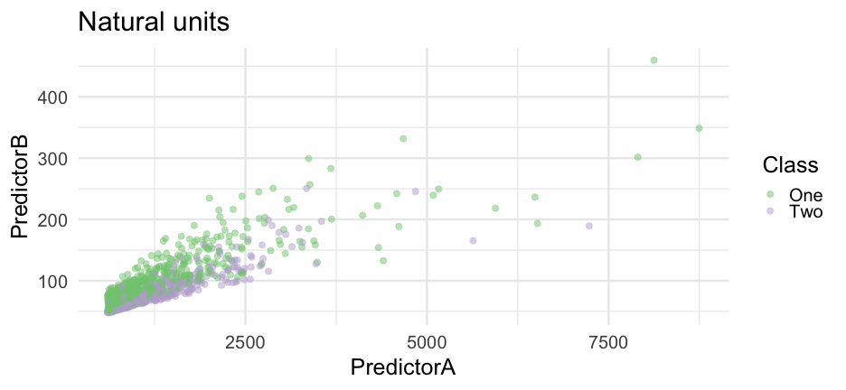
```

![](w5p1-feature-engineering_files/figure-html/sep-seg-plot-1.png)

---
# Inverse transformation

```r
seg %>% 
  mutate(inv_PredictorA = 1/PredictorA, 
         inv_PredictorB = 1/PredictorB) %>% 
ggplot(aes(inv_PredictorA, inv_PredictorB, color = Class)) + 
  geom_point(alpha = .5) + 
  scale_color_brewer(palette = "Accent") +
  labs(title = "Inverse scale")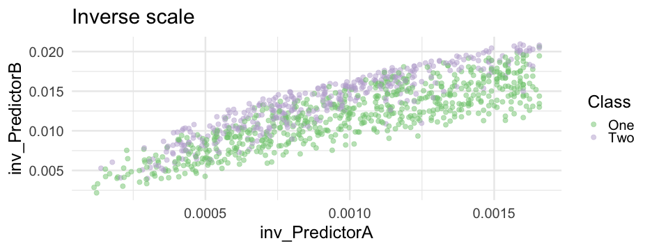
```

![](w5p1-feature-engineering_files/figure-html/seg-inverse-1.png)

---
# Univariate view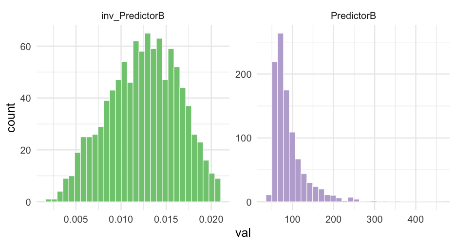

![](w5p1-feature-engineering_files/figure-html/predictora-univariate-1.png)

---
# More general transformation
### Box-Cox transformation
Originally developed as a transformation of the outcome - can help with predictor variables too.

$$
`\begin{equation}
 x^* =
	\begin{cases}
  	\frac{x^\lambda-1}{\lambda}, & \text{if}\ \lambda \neq 0 \\
   	\log\left(x\right), & \text{if}\ \lambda = 0
	\end{cases}
\end{equation}`
$$

--
### Objective

Estimate `$\lambda$` for each  variable to be transformed

--
Technically only for positive values. Use Yeo-Johnson transformation for positive & negative data.

---
# Common `$\lambda$` mappings

* `$\color{#157CAE}{\lambda} = 1$`: No tranformation
* `$\color{#157CAE}{\lambda} = 0$`: log tranformation
* `$\color{#157CAE}{\lambda} = 0.5$`: square root tranformation
* `$\color{#157CAE}{\lambda} = -1$`: inverse

--
### Box Cox transformations

```r
bc <- recipe(Class ~ ., data = seg) %>% 
  step_BoxCox(all_predictors()) %>% 
  prep() 
```

---
class: inverse center middle

# Tidying recipes

---
# tidy
* Once you've created a recipe, you may want to *tidy* it to get more information about a specific step

* In our previous example, we might want to know what `$\lambda$` values were used in the Box-Cox transformation

```r
tidy(bc)
```

```
## # A tibble: 1 x 6
##   number operation type   trained skip  id          
##    <int> <chr>     <chr>  <lgl>   <lgl> <chr>       
## 1      1 step      BoxCox TRUE    FALSE BoxCox_vv7Pc
```

This basically just lists the steps (in this case there's only one). To get the information about the step, we have to specify which number we want to know more about.

---
# Box-Cox Models

```r
tidy(bc, n = 1)
```

```
## # A tibble: 2 x 3
##   terms           value id          
##   <chr>           <dbl> <chr>       
## 1 PredictorA -0.8571484 BoxCox_vv7Pc
## 2 PredictorB -1.091284  BoxCox_vv7Pc
```

We can see that the `$\lambda$` values used was were very close to -1 for each variable, which is close to an inverse transformation.

---
# Backing up a bit
How do we estimate `$\lambda$`?

--
Complicated mathy stuff. But conceptually - find the value the minimizes the difference between the transformed values a theoretical normal distribution

---
# Example

```r
lambdas <- c(-1, -0.5, 0, 0.5, 1)
names(lambdas) <- lambdas

lambda_transforms <- map_df(lambdas, ~ {
  if(.x == 0) {
    log(seg$PredictorB)
  } else {
   (seg$PredictorB^.x - 1) / .x 
  }
})

lambda_d <- seg %>% 
  select(raw = PredictorB) %>% 
  bind_cols(lambda_transforms)

head(lambda_d)
```

```
## # A tibble: 6 x 6
##         raw      `-1`   `-0.5`      `0`    `0.5`       `1`
##       <dbl>     <dbl>    <dbl>    <dbl>    <dbl>     <dbl>
## 1 154.8988  0.9935442 1.839304 5.042772 22.89167 153.8988 
## 2  84.56460 0.9881747 1.782512 4.437516 16.39180  83.56460
## 3 101.0911  0.9901079 1.801082 4.616022 18.10881 100.0911 
## 4  68.71062 0.9854462 1.758722 4.229904 14.57837  67.71062
## 5  73.40559 0.9863771 1.766565 4.296000 15.13541  72.40559
## 6  79.47569 0.9874175 1.775657 4.375451 15.82983  78.47569
```

---
# Move to long

```r
lambda_d %>% 
  pivot_longer(-raw)
```

```
## # A tibble: 5,045 x 3
##          raw name        value
##        <dbl> <chr>       <dbl>
##  1 154.8988  -1      0.9935442
##  2 154.8988  -0.5    1.839304 
##  3 154.8988  0       5.042772 
##  4 154.8988  0.5    22.89167  
##  5 154.8988  1     153.8988   
##  6  84.56460 -1      0.9881747
##  7  84.56460 -0.5    1.782512 
##  8  84.56460 0       4.437516 
##  9  84.56460 0.5    16.39180  
## 10  84.56460 1      83.56460  
## # … with 5,035 more rows
```

---
# Compare to theoretical quantiles

```r
lambda_d %>% 
  pivot_longer(-raw) %>% 
  ggplot(aes(sample = value)) +
  geom_qq_line() +
  stat_qq(aes(color = name)) +
  facet_wrap(~name, scales = "free_y")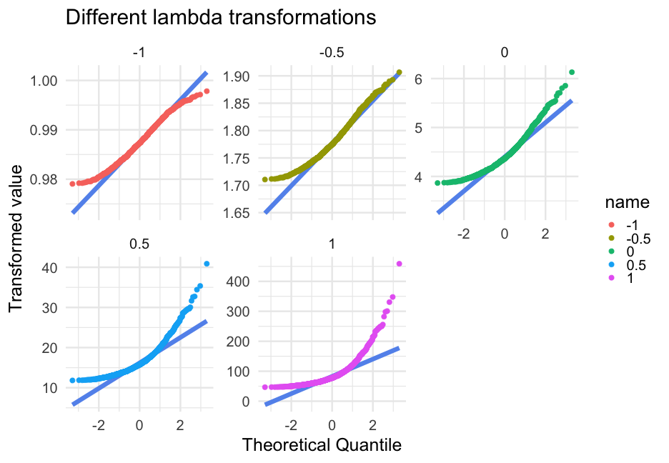
```

---

![](w5p1-feature-engineering_files/figure-html/plot-lambdas-eval-1.png)

---
## More complicated transformations
* Nonlinear transformations may help improve performance

+ Polynomials w/`step_poly`

- Note, these are orthogonal polynomials by default

+ Natural- or B-spline basis functions w/`step_ns` or `step_bs`
  
      - If you're interested in splines, or more generally, GAMs, I highly recommend [Noam Ross's free course](https://noamross.github.io/gams-in-r-course/) to get you started.

---
# Quick example

```r
airquality <- airquality %>% 
  mutate(date = lubridate::make_date(month = Month, day = Day))

ggplot(airquality, aes(date, Temp)) +
  geom_point(color = "gray70")
```

![](w5p1-feature-engineering_files/figure-html/plot-raw-1.png)

---
# Natural spline basis expansion

```r
spline_rec <- recipe(Temp ~ ., airquality) %>%
  step_mutate(date = as.numeric(date)) %>% 
  step_ns(date)

spline_d <- spline_rec %>% 
  prep() %>% 
  juice()
spline_d
```

```
## # A tibble: 153 x 8
##    Ozone Solar.R  Wind Month   Day  Temp  date_ns_1    date_ns_2
##    <int>   <int> <dbl> <int> <int> <int>      <dbl>        <dbl>
##  1    41     190   7.4     5     1    67 0           0          
##  2    36     118   8       5     2    72 0.01004389 -0.006695549
##  3    12     149  12.6     5     3    74 0.02008509 -0.01338702 
##  4    18     313  11.5     5     4    62 0.03012090 -0.02007035 
##  5    NA      NA  14.3     5     5    56 0.04014863 -0.02674146 
##  6    28      NA  14.9     5     6    66 0.05016559 -0.03339627 
##  7    23     299   8.6     5     7    65 0.06016907 -0.04003070 
##  8    19      99  13.8     5     8    59 0.07015639 -0.04664070 
##  9     8      19  20.1     5     9    61 0.08012484 -0.05322217 
## 10    NA     194   8.6     5    10    69 0.09007175 -0.05977105 
## # … with 143 more rows
```

---
# Fit model & make prediction

```r
fit <- lm(Temp ~ date_ns_1 + date_ns_2, data = spline_d)
spline_pred <- spline_d %>% 
  mutate(spline_pred = predict(fit, newdata = spline_d))

spline_pred
```

```
## # A tibble: 153 x 9
##    Ozone Solar.R  Wind Month   Day  Temp  date_ns_1    date_ns_2 spline_pred
##    <int>   <int> <dbl> <int> <int> <int>      <dbl>        <dbl>       <dbl>
##  1    41     190   7.4     5     1    67 0           0              60.74215
##  2    36     118   8       5     2    72 0.01004389 -0.006695549    61.17035
##  3    12     149  12.6     5     3    74 0.02008509 -0.01338702     61.59844
##  4    18     313  11.5     5     4    62 0.03012090 -0.02007035     62.02629
##  5    NA      NA  14.3     5     5    56 0.04014863 -0.02674146     62.45378
##  6    28      NA  14.9     5     6    66 0.05016559 -0.03339627     62.88078
##  7    23     299   8.6     5     7    65 0.06016907 -0.04003070     63.30719
##  8    19      99  13.8     5     8    59 0.07015639 -0.04664070     63.73289
##  9     8      19  20.1     5     9    61 0.08012484 -0.05322217     64.15774
## 10    NA     194   8.6     5    10    69 0.09007175 -0.05977105     64.58163
## # … with 143 more rows
```

---
# Plot predictions

```r
spline_pred %>% 
  mutate(date = lubridate::make_date(month = Month, day = Day)) %>% 
  ggplot(aes(date, Temp)) +
  geom_point(color = "gray70") +
  geom_line(aes(y = spline_pred),
            color = "#4f8dde")
```

![](w5p1-feature-engineering_files/figure-html/plot-preds-1.png)

---
# Increase wiggliness
### Increase the degrees of freedom

```r
spline_rec2 <- recipe(Temp ~ date, airquality) %>%
  step_mutate(date = as.numeric(date)) %>% 
  step_ns(date, deg_free = 7)

spline_d2 <- spline_rec2 %>% 
  prep() %>% 
  juice()
names(spline_d2)
```

```
## [1] "Temp"      "date_ns_1" "date_ns_2" "date_ns_3" "date_ns_4" "date_ns_5"
## [7] "date_ns_6" "date_ns_7"
```

---
# Fit new model

```r
fit2 <- lm(Temp ~ ., data = spline_d2)
spline_pred2 <- spline_d2 %>% 
  mutate(spline_pred = predict(fit2, newdata = spline_d2),
         date = airquality$date) 
```

---
# Plot new predictions

```r
spline_pred2 %>% 
  ggplot(aes(date, Temp)) +
  geom_point(color = "gray70") +
  geom_line(aes(y = spline_pred),
            color = "#4f8dde")
```

![](w5p1-feature-engineering_files/figure-html/plot-preds2-1.png)

---
# One more time
### Just for fun

```r
spline_rec3 <- recipe(Temp ~ date, airquality) %>%
  step_mutate(date = as.numeric(date)) %>% 
  step_ns(date, deg_free = 20)

spline_d3 <- spline_rec3 %>% 
  prep() %>% 
  juice()

fit3 <- lm(Temp ~ ., data = spline_d3)
spline_pred3 <- spline_d3 %>% 
  mutate(spline_pred = predict(fit3, newdata = spline_d3),
         date = airquality$date) 
```

---

```r
spline_pred3 %>% 
  ggplot(aes(date, Temp)) +
  geom_point(color = "gray70") +
  geom_line(aes(y = spline_pred),
            color = "#4f8dde")
```

![](w5p1-feature-engineering_files/figure-html/last-spline-plot-1.png)

---
# Finishing up on splines
* The default for `step_ns` is equivalent to `splines::ns(x, df = 2)`

+ Hyperparameter that can be tuned: see [here](https://tidymodels.github.io/tune/articles/getting_started.html) for an example.
  
  + You probably want to tune variables separately (otherwise the smooth is constrained to be equal)

* Could easily be a course on its own (and is)

* Really powerful and actually can be pretty interpretable

* Can be thought of as a feature engineering consideration (as it is through recipes) rather than a model fitting procedure alone

* Splines themselves are on a predictor-by-predictor basis, but can be extended to multivariate models with generalized additive models (GAMs)

---
class: inverse center middle
# Principal Components Analysis

---
# Collapsing data w/PCA
* For some models (e.g., linear regression) highly correlated variables can reduce predictive accuracy. Collapsing variables may help.

* Basically a way to take a whole bunch of variables and reduce them down to just a few, which carry most of the same information as the raw data

* Can help reduce overfitting, but if this is your primary concern, regularizatoin methods are probably better

--
.bolder[.b[Goal]]: Identify a small number of dimensions (components) that account for .r[X].b[%] of the variation captured by .ital[.bolder[all]] of the variables

---
# Recipe steps to check
* Data are [tidy](https://www.jstatsoft.org/article/view/v059i10) .g[Probs fix before recipe steps]

* No missing data

* All numeric data (so need to use dummy coding, etc)

* Numeric data should be standardized (centered & scaled)

---
# Get ready for PCA
Note, this is the same recipe we had before, except I've encoded and imputed missing data

```r
rec <- recipe(score ~ ., train) %>% 
  step_mutate(tst_dt = lubridate::mdy_hms(tst_dt)) %>% 
  update_role(contains("id"), sch_name, ncessch, new_role = "id vars") %>% 
  step_zv(all_predictors()) %>% 
* step_unknown(all_nominal()) %>%
* step_medianimpute(all_numeric(), -all_outcomes(), -has_role("id vars")) %>%
  step_center(all_numeric(), -all_outcomes(), -has_role("id vars")) %>% 
  step_scale(all_numeric(), -all_outcomes(), -has_role("id vars")) %>% 
  step_dummy(all_nominal(), -has_role("id vars"))
```

---
# Retain 80% of the variance

```r
rec80 <- rec %>% 
  step_pca(all_numeric(), -all_outcomes(), -has_role("id vars"), 
           threshold = .80)

rec80 %>% 
  prep() %>% 
  tidy()
```

```
## # A tibble: 8 x 6
##   number operation type         trained skip  id                
##    <int> <chr>     <chr>        <lgl>   <lgl> <chr>             
## 1      1 step      mutate       TRUE    FALSE mutate_uhixw      
## 2      2 step      zv           TRUE    FALSE zv_3vWwp          
## 3      3 step      unknown      TRUE    FALSE unknown_yVUgc     
## 4      4 step      medianimpute TRUE    FALSE medianimpute_Rc0sD
## 5      5 step      center       TRUE    FALSE center_Q9i55      
## 6      6 step      scale        TRUE    FALSE scale_Sn3mL       
## 7      7 step      dummy        TRUE    FALSE dummy_bTSdq       
## 8      8 step      pca          TRUE    FALSE pca_GLbC5
```

---
# Which variable went to which?

```r
rec80 %>% 
  prep() %>% 
  tidy(n = 8)
```

```
## # A tibble: 6,561 x 4
##    terms                                     value component id       
##    <chr>                                     <dbl> <chr>     <chr>    
##  1 enrl_grd                            1.912533e-4 PC1       pca_GLbC5
##  2 lat                                -1.957178e-3 PC1       pca_GLbC5
##  3 lon                                 1.083956e-6 PC1       pca_GLbC5
##  4 p_american_indian_alaska_native    -1.314160e-4 PC1       pca_GLbC5
##  5 p_asian                            -1.632283e-3 PC1       pca_GLbC5
##  6 p_native_hawaiian_pacific_islander -1.384953e-3 PC1       pca_GLbC5
##  7 p_black_african_american           -1.347631e-3 PC1       pca_GLbC5
##  8 p_hispanic_latino                  -1.707349e-3 PC1       pca_GLbC5
##  9 p_white                             2.613973e-3 PC1       pca_GLbC5
## 10 p_multiracial                      -2.537467e-4 PC1       pca_GLbC5
## # … with 6,551 more rows
```

Note - we have too many features and too many components to produce many meaningful plots, but you could look at subsamples.

---
### How many PCAs to retain 95% of the variance?

```r
rec %>% 
  step_pca(all_numeric(), -all_outcomes(), -has_role("id vars"), 
           threshold = .95) %>% 
  prep() %>% 
  juice() %>% 
  select(id, starts_with("PC"), score)
```

```
## # A tibble: 142,170 x 15
##       id     PC01       PC02        PC03       PC04         PC05       PC06
##    <dbl>    <dbl>      <dbl>       <dbl>      <dbl>        <dbl>      <dbl>
##  1     1 3.912798  3.651945  -1.456787   -0.4358499 -1.620380e+0  0.1799292
##  2     2 4.210309 -1.924723  -0.4836048  -0.1317212  6.193062e-1  0.7882637
##  3     5 3.908650  1.509492  -2.814445    1.934177   5.269454e-2 -1.711811 
##  4     7 3.901849 -1.546685   0.6916342   0.7535638 -2.466424e+0 -0.4757124
##  5    10 4.215300 -0.6347256  0.2479699   1.555374  -2.908392e-1  0.3576653
##  6    12 3.982035  0.8435940  0.2888210   1.384601  -7.181826e-1  0.2099972
##  7    13 4.170530 -1.379940  -0.3243078   1.798536  -4.915138e-4  0.6429018
##  8    14 4.218798 -1.301757   0.09514081  0.9060468 -2.277564e+0 -0.7943368
##  9    17 4.187044 -1.680436   0.3212928   1.000362  -2.047639e+0 -0.4962436
## 10    21 4.120930 -0.6330739  0.2432836   1.546083  -3.004679e-1  0.3534600
## # … with 142,160 more rows, and 8 more variables: PC07 <dbl>, PC08 <dbl>,
## #   PC09 <dbl>, PC10 <dbl>, PC11 <dbl>, PC12 <dbl>, PC13 <dbl>, score <dbl>
```

---
# One last note
This has obviously been a .b[.ital[very]] quick discussion of PCA.

We're thinking of it primarily as a feature engineering approach.

Check out [Julia Silge's post](https://juliasilge.com/blog/best-hip-hop/) for more on PCA, continuing through a tidymodels view.

---
class: inverse center middle
# Wrapping up

---
# Feature engineering (FE)
* Almost endless possibilities

* Probably the most "art" part of ML

* Amazing FE and a simple model will regularly beat poor FE and a fancy model

* {recipes} is a great package to do a lot of the work for you

--
Remember - it creates a .b[blueprint]! This means, we can (and should) apply the blueprint (recipe) to each fold when we're using `$k$`-fold CV

---
# Full recipe
### 95% of variance in PCA

```r
rec <- recipe(score ~ ., train) %>% 
  step_mutate(tst_dt = lubridate::mdy_hms(tst_dt)) %>% 
  update_role(contains("id"), sch_name, ncessch, new_role = "id vars") %>% 
  step_zv(all_predictors()) %>% 
  step_unknown(all_nominal()) %>% 
  step_medianimpute(all_numeric(), -all_outcomes(), -has_role("id vars")) %>% 
  step_center(all_numeric(), -all_outcomes(), -has_role("id vars")) %>% 
  step_scale(all_numeric(), -all_outcomes(), -has_role("id vars")) %>% 
  step_dummy(all_nominal(), -has_role("id vars")) %>% 
  step_pca(all_numeric(), -all_outcomes(), -has_role("id vars"), 
           threshold = .95)

prepped_rec <- prep(rec)
```

---
# Apply in CV
* Note the transformations are being conducted .b[for each fold], which ensures there is no data leakage

```r
cv <- vfold_cv(train)
cv_baked <- cv %>% 
  mutate(baked = map(splits, ~bake(prepped_rec, .x)))
cv_baked
```

```
## #  10-fold cross-validation 
## # A tibble: 10 x 3
##    splits               id     baked                  
##    <list>               <chr>  <list>                 
##  1 <split [128K/14.2K]> Fold01 <tibble [127,953 × 22]>
##  2 <split [128K/14.2K]> Fold02 <tibble [127,953 × 22]>
##  3 <split [128K/14.2K]> Fold03 <tibble [127,953 × 22]>
##  4 <split [128K/14.2K]> Fold04 <tibble [127,953 × 22]>
##  5 <split [128K/14.2K]> Fold05 <tibble [127,953 × 22]>
##  6 <split [128K/14.2K]> Fold06 <tibble [127,953 × 22]>
##  7 <split [128K/14.2K]> Fold07 <tibble [127,953 × 22]>
##  8 <split [128K/14.2K]> Fold08 <tibble [127,953 × 22]>
##  9 <split [128K/14.2K]> Fold09 <tibble [127,953 × 22]>
## 10 <split [128K/14.2K]> Fold10 <tibble [127,953 × 22]>
```

---
class: inverse 
# Next class
We'll review a bit of this, discuss any points of confusion, and get started on the lab.