class: center, middle, inverse, title-slide # Inference versus prediction ## And a basic intro to some topics in ML ### Daniel Anderson & Joe Nese ### Week 2, Class 1 --- # Agenda * Modeling for inference vs prediction -- * Train and test datasets -- * Objective functions (briefly) -- * Bias-Variance tradeoff of and overfitting -- * Supervised vs unsupervised learning -- * Regression vs Classification --- # Check in and announcements * How's the start of your term going? * Anything unclear or that you'd like to discuss? * Please remember to email us with your group! + Ideally, please have this settled by the end of today ---  --- 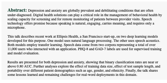 [RSVP Here](https://urldefense.com/v3/__https:/oregon.qualtrics.com/jfe/form/SV_bx4862NYcmcnNg9__;!!C5qS4YX3!XOuDAPFLxffMTm3Bs5-MN0EESFaOjwxJj5DQioA89VGClJ10O5RhT0dB6ihwsd4$) --- class: inverse center middle # Inference vs Prediction --- # What's the difference? Focus of most stats classes is on inference -- ### Example RQ's * What is the relation between the proportion of students eligible for free/reduced price lunch and a school's Annual Performance Index? -- * What is the effect of a reading intervention for struggling readers, as compared to treatment as usual? -- * To what extent does the effect of internalizing/externalizing behavior on sexual risk depend upon their adverse childhood experiences? --- # Standard errors * One of the defining features of modeling for inference is the estimation of a standard error for a given estimate -- * How certain are we of the population-level estimate? --- # Prediction * Rather than inferring population-level values, the focus shifts to building a "machine" that produces predictions for us on new (unseen) data -- * Less focus on population-level values, or even model interpretability. -- * Primary focus - how well does our model perform? -- * Standard errors of your coefficients are generally not as important as the model prediction error --- # Another way to think of it ### Our linear regression model `$$\color{#157CAE}{\text{Y}_{i}} = \text{X}_{i} \color{#DB1593}{\beta} + e_i$$` -- When modeling for inference, we want an unbiased (consistent) and precise estimate `\(\color{#DB1593}{\hat\beta}\)`. -- For prediction, we shift our focus to accurately estimating outcomes. -- In other words, how can we best construct `\(\color{#157CAE}{\hat{\text{Y}}_{i}}\)`? --- ## ... so? So we want "nice"-performing estimates `\(\hat y\)` instead of `\(\hat\beta\)`. .r[Q]: Can't we just use the same methods (_i.e._, OLS)? -- .b[A]: It depends. -- How well does your .bolder[.r[linear]]-regression model approximate the underlying data? (And how do you plan to select your model?) --- # Why might we want to do this? * Forecasting is useful -- * What is the likelihood that a kindergarten student will be reading on "grade-level" by third grade? -- * What is the likelihood that a given student has a disability? -- * What is the likelihood that a given student will drop out of high-school? -- ### In each case: * Build a predictive model * Use the model to forecast/predict * Update the forecast/prediction as more data are collected * Taylor instruction/intervention to these forecasts --- # Example forecast plot 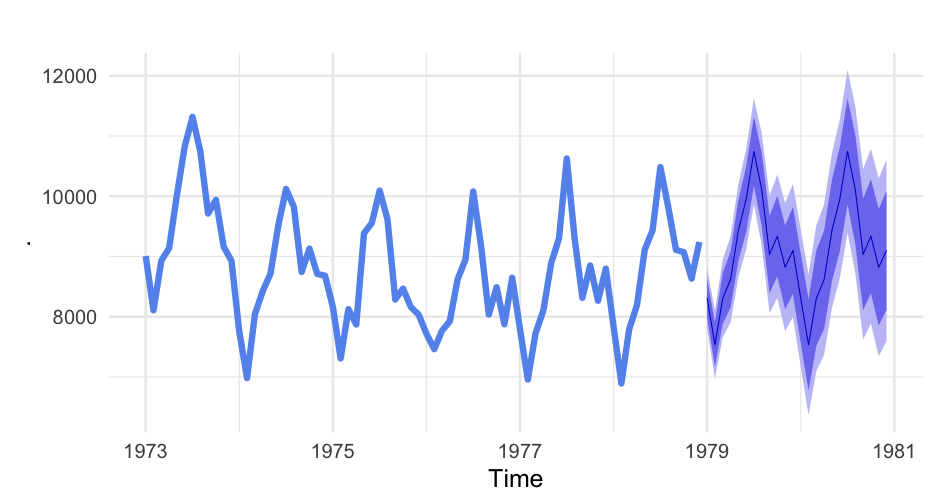<!-- --> --- # A warning  --- * Lots of misunderstanding out there about what predictive modeling is, and many people will disparage it -- * .bolder[My view:] + these people generally have an incomplete (at best) understanding of predictive modeling + Often have antiquated views of the techniques used in predictive modeling (i.e., not about maxing out `\(R^2\)`) -- ### Bottom line * Predictive modeling has been used with enormous success * These models are used in production business environments all the time * These modeling techniques impact all of our lives on a daily basis --- class: inverse center middle # The antiquated method --- # Stepwise regression * Often when people bad-talk predictive modeling, it's because they're thinking of stepwise regression -- ### Basic approach * Throw a bunch of variables at a problem, only keep those that are significant --- # Approaches * **Forward selection:** Start with no variables, add one at a time, but only keep if significant -- * **Backward selection:** Start with all variables, remove one at a time based on the variable that is "least significant" -- * **Stepwise selection:** Sequentially add predictor variables based on "most significant". After each addition, cycle through and remove non-significant variables -- ### Goal * Find the optimal subset of variables that could be used to predict the outcome --- # Reasons for critique * `\(p\)` values were not designed for variable selection decisions! * Even if we wanted to use them, why use `\(\alpha = 0.05\)`, rather than what works best for the given problem? -- ### More importantly * People use this model **for inference** which is straight-up bonkers -- ### Why are we talking about this? * It actually can still be an okay method if all you care about is variable selection. * Make you aware that others may use it inappropriately, and to caution you (in the strongest way possible) not to use it for inference. --- # Stepwise criteria * Applying different criteria (forward, backward, etc.) can lead to different "optimal" variable combinations -- * From a predictive modeling framework, this isn't really a big deal - we only care about which model performs best. -- * From an inference perspective, it's a REALLY big deal - that's why we don't use these models for inference + Little to no theory guiding decisions, except which variables will be included in the automatic procedure (which is often all available variables) --- class: inverse center middle # How do we determine "performance" --- # Model performance criteria * If the primary concern is prediction, what do we care about the most? -- .center[### How close our predictions to the observed data?] -- .Large[🤨] * Wait, isn't that basically the same thing as residual variance? -- ### No! * Why? We want to know how far off our model is for .bolder[.b[cases outside our sample]!] --- # Test/Train datasets * Our goal is to maximize .bolder[.b[out-of-sample]] predictive accuracy. How can we get an estimate of that? Leave out part of the sample. -- 1. Split the raw data into "training" and "test" datasets -- 2. Build a model on the training dataset -- 3. Do everything you can to make the model the "best" you can -- 4. When you've settled on a .bolder[final] model, use the parameter estimates to predict the outcome on the test data -- 5. Use an objective function to evaluate how far off your predictions were from the real values --- # Quick example ```r library(tidyverse) set.seed(8675309) train <- mtcars %>% sample_frac(.8) test <- anti_join(mtcars, train) nrow(train) ``` ``` ## [1] 26 ``` ```r nrow(test) ``` ``` ## [1] 6 ``` --- # Fit model(s) * Only use the training data ```r m1 <- lm(mpg ~ hp, train) m2 <- lm(mpg ~ hp + disp, train) m3 <- lm(mpg ~ hp + disp + cyl, train) sundry::aic_weights(m1, m2, m3) ``` ``` ## predictors delta weight ## 3 hp + disp + cyl 0.0000000 0.58 ## 2 hp + disp 0.6834108 0.41 ## 1 hp 11.5038955 0.00 ``` -- ### Settle on a model It's basically a toss-up between `m2` and `m3`. I'll go with the more parsimonious model. --- # Predict new cases ```r test <- test %>% mutate(pred_mpg = predict(m2, newdata = test)) test ``` ``` ## mpg cyl disp hp drat wt qsec vs am gear carb pred_mpg ## 1 21.0 6 160.0 110 3.90 2.620 16.46 0 1 4 4 23.53699 ## 2 24.4 4 146.7 62 3.69 3.190 20.00 1 0 4 2 25.15279 ## 3 27.3 4 79.0 66 4.08 1.935 18.90 1 1 4 1 27.27787 ## 4 15.8 8 351.0 264 4.22 3.170 14.50 0 1 5 4 13.48171 ## 5 19.7 6 145.0 175 3.62 2.770 15.50 0 1 5 6 22.43303 ## 6 21.4 4 121.0 109 4.11 2.780 18.60 1 1 4 2 24.84235 ``` -- Consider *how* you want to evaluate how well your model performed (what objective function to use). -- In this case, we'll look at the root mean square residual (RMSE), which we want to minimize --- # Calculate differences ```r test %>% mutate(diff = pred_mpg - mpg) ``` ``` ## mpg cyl disp hp drat wt qsec vs am gear carb pred_mpg diff ## 1 21.0 6 160.0 110 3.90 2.620 16.46 0 1 4 4 23.53699 2.53699114 ## 2 24.4 4 146.7 62 3.69 3.190 20.00 1 0 4 2 25.15279 0.75278654 ## 3 27.3 4 79.0 66 4.08 1.935 18.90 1 1 4 1 27.27787 -0.02213242 ## 4 15.8 8 351.0 264 4.22 3.170 14.50 0 1 5 4 13.48171 -2.31828902 ## 5 19.7 6 145.0 175 3.62 2.770 15.50 0 1 5 6 22.43303 2.73302814 ## 6 21.4 4 121.0 109 4.11 2.780 18.60 1 1 4 2 24.84235 3.44235070 ``` -- What's the average difference? -- <img src="https://datainsure.com/wp-content/uploads/2018/04/ZERO-01.png" height="175px" /> --- # What do we do? -- * Square then average the values -- ### Mean square error .Large[ $$ MSE = \frac{1}{n}\sum(y\_i - \hat{y\_i})^2 $$ ] -- ### Root mean square error .Large[ $$ RMSE = \sqrt{\frac{1}{n}\sum(y\_i - \hat{y\_i})^2} $$ ] --- # Objective function * MSE and RMSE are examples of **objective functions**, **cost functions**, or **loss functions**. There are many of these, which we'll talk more about later in the term. * Goal of ML - optimize (maximize or minimize) the objective function * These are all [similar but not equivalent](https://stats.stackexchange.com/questions/179026/objective-function-cost-function-loss-function-are-they-the-same-thing) terms --- # Evaluate ```r test %>% summarize(mse = mean((pred_mpg - mpg)^2)) ``` ``` ## mse ## 1 5.282864 ``` ```r test %>% summarize(rmse = sqrt(mean((pred_mpg - mpg)^2))) ``` ``` ## rmse ## 1 2.298448 ``` -- * Note, you can only evaluate against the test set once! Otherwise, your test dataset becomes part of your training dataset. -- * Instead, you do this process over and over **with your training dataset** through a process called `\(k\)`-fold cross-validation, which we'll talk about next week. --- ## `\(k\)`-fold CV basics * Split the data into multiple little samples -- * Leave out one piece, try different models on the other pieces, predict on left out piece -- * Evaluate against objective function -- ### Joe will cover this more next week --- class: inverse center middle # Overfitting ### And thinking more about functional form .Large[ $$ \hat{Y} = f(\mathbf{X}) $$ ] --- # Predicting income * Imagine we are trying to predict respondents' income. -- * In this case, the data have been simulated, so .b[we know] the functional form -- .center[ <img src="img/true-functional-form.png" height="350px" /> ] --- # We could fit a linear relation .center[ <img src="img/linear-relation.png" height="450px" /> ] --- # Or a more complex model .center[ <img src="img/spline-good.png" height="450px" /> ] --- # Or a really complicated model .center[ <img src="img/spline-bad.png" height="450px" /> ] --- * The linear model doesn't fit the observed data as well .gray[(it is slightly underfit)] -- * The really complex model model fits the observed data nearly perfectly .gray[(it is overfit)] -- * The middle model fits the observed data well, and matches the underlying function well. -- * We know this because we know the underlying function - usually we do not. --- # Overfitting in action .center[  ] --- class: inverse center middle # Bias-Variance Trade-off --- # Types of errors in prediction <br/> -- ### Bias How well does the model represent the observed data? -- ### Variance How much does the model change from sample to sample? --- # Linear models Tend to have low variance -- ### But also... Can have high bias, if the underlying functional form is not *truly* linear --- # Highly flexible models Tend to have low bias (representing the observed data well) -- ### But also... Can easily overfit, leading to high variance -- ### The goal * Balance the bias-variance trade-off -- * Note, this is an incredibly useful perspective **even if your goal is to model for inference.** --- # More gifs! Why the linear model has low variance  --- Why it may have high bias  --- # A crazy polynomial model Why more complicated models have higher variance  --- Why it may have lower bias  --- # More precise definitions .pull-left[ ### Bias * Difference between the .gray[(average, oftentimes)] prediction of our model and the "true" value * Equivalent to statistical bias * How well the model fit the underlying structure of the data? * Low bias = closer to “truth” * High bias = systematically ignores structure in the data ] -- .pull-right[ ### Variance * Variability of the model predictions for a given point * Variability of predictions if the model were repeated with small differences in the data * Degree that model predictions are influenced by these changes = variance * High variance models generalize to unseen data poorly ] --- background-image:url(https://sebastianraschka.com/images/blog/2016/model-evaluation-selection-part2/visual_bias_variance.png) background-size: contain --- background-image:url(https://bradleyboehmke.github.io/HOML/02-modeling-process_files/figure-html/modeling-process-bias-model-1.png) background-size: contain # Low variance - moderate bias .footnote[https://bradleyboehmke.github.io/HOML/process.html#bias-var] --- background-image:url(https://bradleyboehmke.github.io/HOML/02-modeling-process_files/figure-html/modeling-process-variance-model-1.png) background-size: contain # High variance - low bias .footnote[https://bradleyboehmke.github.io/HOML/process.html#bias-var] --- # General model characteristics ### Less flexible, but low variance * Linear regression * Ridge/lasso * Partial least squares -- ### More flexible, but higher variance * `\(KNN\)` * Decision trees * Neural networks --- background-image:url(https://cdn.analyticsvidhya.com/wp-content/uploads/2020/08/Copy-of-Add-a-subheading5.png) background-size: contain .footnote[https://www.analyticsvidhya.com/blog/2020/08/bias-and-variance-tradeoff-machine-learning/] --- # Strategies for optimizing ### Hyperparameter tuning Many machine learning models include parameters that must be set by the analyst, which control the flexibility of the model ### Regularization Reduce how much the model learns. Many different strategies, including * Penalties on model fit + Highly complex models are penalized higher, leading to less likelihood of being selected * Shrinkage + Systematically reduce the influence of a given parameter, or sets of parameters * Dropout + Randomly drop trees/nodes in the learning process --- class: inverse center middle # Regression versus classification -- # Supervised versus unsupervised learning --- # What are you trying to predict? * Continuous (or approximately continuous) response variable? + Regression problem -- * Categorical response variable? + Classification problem -- * Simplest examples: + Linear regression -- .b[regression] -- + Logistic regression -- .r[classification] -- + Ordinal or multinomial regression -- .r[classification] --- # Supervised/unsupervised * Supervised: You have .b[*labeled*] data -- ### What does labeled mean? -- * Just that you have scores or classifications or whatever for the thing you're trying to get the machine to "learn". -- * Unsupervised: No labels --- # Supervised/unsupervised * Supervised learning is fairly straightforward - you have values of some outcome for a sample. Try to build a model to predict the values people outside of your sample would have. * Unsupervised - Clustering problems - Latent class/mixture modeling - No way to "know" a case belongs to a certain class/response level --- # Pop quiz <div class="countdown" id="timer_5f7b47ad" style="top:0;right:0;" data-warnwhen="0"> <code class="countdown-time"><span class="countdown-digits minutes">05</span><span class="countdown-digits colon">:</span><span class="countdown-digits seconds">00</span></code> </div> <br/> Talk with your neighbor to determine whether each of the following is a .b[regression] or .r[classification] problem .bolder[AND] whether it is a .b[supervised] or .r[unsupervised] problem. Note - there is no "correct" answer for some of these, it depends on how it's framed * Develop an algorithm that determines if students will be reading on grade level by the third grade, according to a statewide test. * Predict which students will be at risk for reading difficulties. * Estimate who is most at risk to drop out of high school. * Determine specific objects in an image * Decode handwriting to text * Estimate the likelihood of having a learning disability --- class: inverse # Next class Ethics in Machine Learning. Guest lecture: [Sondra Stegenga](https://www.linkedin.com/in/sondra-stegenga/) <br/> .center[]