class: center, middle, inverse, title-slide # Neural net babysteps ## An intro with Keras and Tensorflow in R ### Daniel Anderson ### Week 10, Class 2 --- # Agenda * Some house cleaning sort of stuff * Intro to neural nets/deep learning * Estimation with keras * Challenge: Tweaking model capacity * Learning rates (and optimizers with adaptive learning rates) --- # Acknowledgements, Resources, & Disclaimers * Most of this content comes from a deep learning training I attended with Bradley Boehmke * All of the content from that training [is freely available](https://github.com/rstudio-conf-2020/dl-keras-tf) * The [keras](https://keras.rstudio.com) website is also a great place to start learning * I'm very new to this .g[but it's very cool] --- class: inverse center middle # Before we really get started --- # Reading the docs There are some kind of weird conventions that made the docs a little more difficult for me to read than I would expect. ### Object unpacking ```r library(zeallot) my_name <- c("Daniel", "Anderson") c(first, last) %<-% my_name first ``` ``` ## [1] "Daniel" ``` ```r last ``` ``` ## [1] "Anderson" ``` --- # Tensors When you read about tensors, you should just think vectors, matrices, and arrays -- * 1D Tensor = vector -- * 2D Tensor = matrix -- * 3/4/5D Tensor = 3/4/5-dimensional array --- # Visual examples: 1D Tensor  --- # Visual examples: 2D Tensor 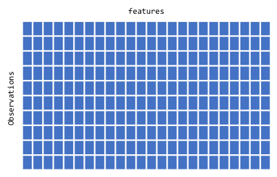 --- # Visual examples: 3D Tensor 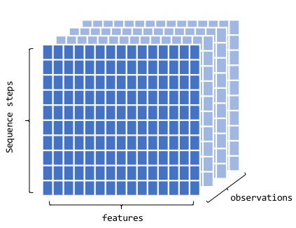 --- # Visual examples: 4D Tensor 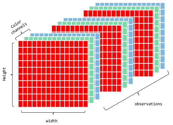 --- # Visual examples: 5D Tensor <img src="img/5D_tensor.jpg" width="60%" /> --- class: inverse center middle # Intro to neural nets & deep learning --- # What is deep learning? * Neural net with two or more hidden layers -- <img src="https://miro.medium.com/max/1400/1*3fA77_mLNiJTSgZFhYnU0Q@2x.png" width="80%" /> .footnote[Image source: https://medium.com/@ksusorokina/image-classification-with-convolutional-neural-networks-496815db12a8] --- # Deep learning use cases * Voice/facial recognition * Flaw detection (engine sounds) * Recommender algorithms (e.g., Amazon, Spotify, Netflix) * Machine vision (e.g., object detection) * Feature extraction -- One of my favorites - the scanner function in the [goodreads](https://www.goodreads.com) mobile app --- # Why deep learning .pull-left[ * Automatic feature extraction * Flexibility * Tends to work better than many alternative methods for high-dimensional and unstructured data - texts, images, audio recording ] -- .pull-right[ 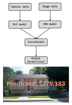 ] --- # What is it? * I like to think of neural nets as, basically, linear regression -- * Linear regression models can be fit through a neural net framework -- ### The following are equivalent $$ y\_{i} = \alpha + b\_{1}x\_{1i} + b\_{2}x\_{2i} + b\_{3}x\_{3i} + e $$ <img src="img/perceptron.png" width="50%" /> --- # Vocabulary * .b[Coefficients] in regression = .r[weights] in neural nets -- * .b[Intercept] in regression = .r[bias] in neural nets -- * .b[Link function] in regression = .r[Activation function] in neural nets --- # Feed forward network * Fundamental building block for most neural network models -- * Implemented in *{keras}* with `layer_dense` --- # A basic model ```r library(keras) network <- keras_model_sequential() %>% layer_dense() %>% # hidden layer layer_dense() # output layer ``` --  --- # A deeper model ```r network <- keras_model_sequential() %>% layer_dense() %>% # hidden layer 1 layer_dense() %>% # hidden layer 2 layer_dense() %>% # hidden layer 3 layer_dense() # output layer ``` --  --- # Arguments to the layers * `units`: The number of perceptrons in the layer * `activation`: The activation function for the perceptrons in the layer * `input_shape`: The number of columns in the design matrix (i.e., matrix including all the predictor variables) -- The `units` and `activation` should be specified for each layer, but the `input_shape` only needs to be specified for the first layer - subsequent layers will layers will be determined automatically --- # Activation Each perceptron goes through a two-step process  --- # Linear transformation Multiply the weights by the `\(x_i\)` values and sum (i.e., linear regression)  --- # Activation Transform the output according to a function  --- # Transformations * The most common activation functions for .b[hidden layers] is ReLU (which we'll get to momentarily), but others exist * For output layers: + Regression problems: Linear/identity activation function + Binary classification: Sigmoidal activation function + Multiclass classification: Softmax transformation (transforms to probability of each class) -- .center[ <img src="img/sigmoid.jpg" width="40%" /> ] --- # Activation functions for hidden layers * Must be non-linear (otherwise the multiple layers collapse to a single layer, see [here](https://ai.stackexchange.com/questions/5493/what-is-the-purpose-of-an-activation-function-in-neural-networks/5521#5521) for an explanation) * ReLU is most common and should be your default * Other options include sigmoid and tanh --- # ReLU Rectified Linear Unit: Super simple - more so than other activation functions $$ ReLU = max(0, z) $$ <!-- --> --- # How does this work? * Remember, we have densely connected perceptrons * Multiple ReLU activations can result in highly complex shapes  --- # Benefits of ReLU Sparse activation * Sigmoid/tanh activations will essentially never be exactly zero, meaning all neurons will always "fire" * "Lighter" networks * More computationally efficient than other activation functions -- ### However * "dying ReLu problem" (perceptrons stop responding) when we would like them not to * Should .r[never] be used for output layers - only hidden layers --- # How neural nets estimate  --- # How neural nets estimate  --- # How neural nets estimate 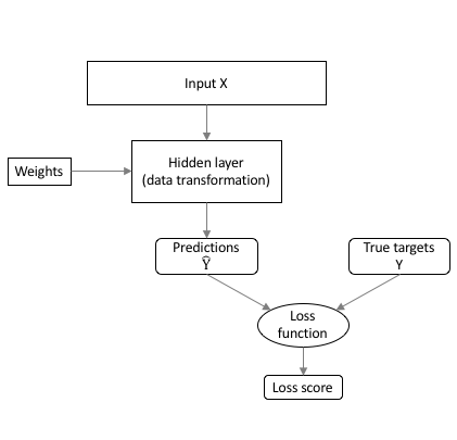 --- # How neural nets estimate 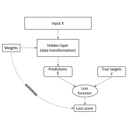 --- # Backpropogation The weights are updated iteratively to minimize the loss score 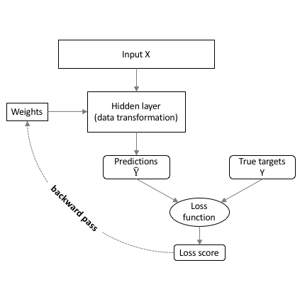 --- # Optimization We have to use an optimizer to determine the best weights to minimize the loss score 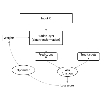 --- # Batch Gradient Descent This is what we talked about last week <!-- --> --- # Stochastic Gradient Descent <!-- --> Gradient is evaluated and updated from a single randomly selected observation --- # Mini-batch Gradient Descent <!-- --> --- # Pros/Cons .pull-left[ .Large[Batch GD] * .gr[Fewer updates] * .gr[Often leads to quicker convergence] * .r[Scales poorly] * .r[Prone to local minima] .Large[Stochastic GD] * .gr[Noisy gradient - avoids local minima] * .r[computationally inefficient] * .r[Noisy gradient can lead to difficulty converging] ] -- .pull-right[ .Large[Mini-batch GD] * .gr[Balances prior two] * .r[One more hyperparameter] * Usually used with `\(2^s\)` ] --- # Epochs Number of times the algorithm goes through the entire training data <!-- --> --- class: inverse center middle # Let's estimate! Launch R Studio, pull up the script I've prepared for you, and let's do it together! --- # Linear regression First, let's use a neural net to replicate a linear regression problem ### Simulate some data ```r library(tidyverse) n <- 1000 # n observations b <- 30 # intercept a <- 5 # slope set.seed(123) (sim <- tibble( x = runif(n, min = -1, max = 1), y = b + a*x + rnorm(n) )) ``` ``` ## # A tibble: 1,000 x 2 ## x y ## <dbl> <dbl> ## 1 -0.4248450 27.27388 ## 2 0.5766103 31.88935 ## 3 -0.1820462 30.11655 ## 4 0.7660348 34.58124 ## 5 0.8809346 32.89551 ## 6 -0.9088870 25.36042 ## 7 0.05621098 29.38511 ## 8 0.7848381 31.85344 ## 9 0.1028700 30.66447 ## 10 -0.08677053 29.48694 ## # … with 990 more rows ``` --- # Visualize relation ```r ggplot(sim, aes(x, y)) + geom_point() + geom_smooth(method = "lm") ``` <!-- --> --- # Estimate w/OLS ```r ols_model <- lm(y ~ x, sim) coef(ols_model) ``` ``` ## (Intercept) x ## 30.011774 4.970831 ``` ```r sigma(ols_model) ``` ``` ## [1] 1.001877 ``` --- # Estimate w/Keras * We need to specify `x` as a matrix * We'll fit a feed-forward sequential neural net with a single perceptron (no hidden layers) ```r x <- matrix(sim$x, ncol = 1) library(keras) mod <- keras_model_sequential() %>% layer_dense(units = 1, activation = "linear", input_shape = ncol(x)) ``` --- # Compile the model * Specify the loss function and optimizer * Note there's no assignment (but it compiles anyway) ```r mod %>% compile(optimizer = "sgd", # stochastic gradient descent loss = "mse") # mean square error ``` --- # Fit * Specify the data, batch size (assuming mini-batch gradient descent), epochs, and validation split * Note - if you run the following more than once, the model will get updated each time (starting from previous best) ```r history <- mod %>% fit(x, sim$y, # data batch_size = 16, # mini-batch size epochs = 20, # n times through full training data validation_split = .2) ``` --- # Check learning ```r plot(history) ``` --- # Compare results .pull-left[ ```r get_weights(mod) coef(ols_model) ``` ] .pull-right[ ```r history sigma(ols_model) ``` ] --- # A more complicated model Simulate data that follow a sin curve ```r set.seed(123) df <- tibble( x = seq(from = -1, to = 2 * pi, length = n), e = rnorm(n, sd = 0.2), y = sin(x) + e ) ``` --- # Visualize relation ```r ggplot(df, aes(x, y)) + geom_point() + geom_line(aes(y = sin(x))) ``` <!-- --> --- # Model capacity Your model capacity is controlled by the model .b[*depth*] (number of layers) and the model .b[*width*] (number of perceptrons in the layer) -- Generally, increasing the depth of a model will result in bigger performance gains than increasing the width of a model --- # Best practices .pull-left[ * Layers are typically *tunnel* or *funnel* shaped * Nodes are powers of 2 (e.g., 4, 8, 16, 32) * Consistent nodes per layer (tunnel) can make tuning easier * Final hidden layer should have more nodes than the output layer ] .pull-right[ <img src="img/model_capacity_depth.png" width="960" height="50%" /><img src="img/model_capacity_funnel.png" width="960" height="50%" /> ] --- # Challenge * Fit a model to the sine wave data * Vary the model capacity (width and depth) and batch size * After each model completes, run the following code to see how close your model was to the true relation * Note: `df` is your simulated data (from 4 slides previous); `model` is your model fit; `x` is the variable from the simulated data ```r df %>% mutate(pred = predict(model, x) %>% as.vector()) %>% ggplot(aes(x, y)) + geom_point() + geom_line(aes(y = sin(x)), color = "cornflowerblue") + geom_line(aes(y = pred), lty = "dashed", color = "red") ``` --- class: inverse center middle # How close did you get? ### And how did you get there? --- # Last topic for today ### Learning rates -- As we talked about with boosted trees, learning rate is an important hyperparameter  --- # Adaptive learning rates Change the learning rate based on the steepness of the gradient .pull-left[ * Simplest approach - add .b[momentum] to the learning rate. Momentum is just a fraction of the previous step added to the current step. * Helps to go "downhill" faster ] .pull-right[  ] --- # Other adaptive LR parameters ### Reduce learning rate on plateau * If no improvements have been made after .b[X] iterations, reduce the learning rate to help find the absolute minimum for that area (i.e., so you don't keep jumping over it) -- * The .b[X] is called the .ital[patience] parameter -- * Can also use callbacks for things like early stopping ```r callback_early_stopping(patience = 3, restore_best_weights = TRUE, min_delta = 0.0001) ``` --- # Example ```r x <- matrix(df$x, ncol = 1) sin_mod <- keras_model_sequential() %>% layer_dense(units = 256, activation = "relu", input_shape = ncol(x)) %>% layer_dense(units = 256, activation = "relu") %>% layer_dense(units = 256, activation = "relu") %>% layer_dense(units = 1, activation = "linear") sin_mod %>% * compile(optimizer = optimizer_sgd(lr = 0.01, momentum = 0.9), loss = "mse") history <- sin_mod %>% fit(x, df$y, batch_size = 16, epochs = 50, validation_split = .2, * callbacks = callback_reduce_lr_on_plateau(factor = 0.1, * patience = 5)) ``` --- # Uh oh When we run this code with our previous model specification, we get weird predictions. Why? What happened? ```r df %>% mutate(pred = predict(sin_mod, x) %>% as.vector()) %>% ggplot(aes(x, y)) + geom_point() + geom_line(aes(y = sin(x)), color = "cornflowerblue") + geom_line(aes(y = pred), lty = "dashed", color = "red") ``` --- # We forgot to randomly sort ```r *df2 <- df[sample(seq_len(nrow(df))), ] *x <- matrix(df2$x, ncol = 1) # sin_mod <- keras_model_sequential() %>% layer_dense(units = 256, activation = "relu", input_shape = ncol(x)) %>% layer_dense(units = 256, activation = "relu") %>% layer_dense(units = 256, activation = "relu") %>% layer_dense(units = 256, activation = "relu") %>% layer_dense(units = 1, activation = "linear") sin_mod %>% compile(optimizer = optimizer_sgd(lr = 0.01, momentum = 0.9), loss = "mse") history <- sin_mod %>% fit(x, df2$y, batch_size = 16, epochs = 50, validation_split = .2, callbacks = callback_reduce_lr_on_plateau(factor = 0.1, patience = 5)) ``` <!-- --- --> <!-- # New fit --> <!-- ```{r plot-sin2, echo = FALSE, eval = FALSE} --> <!-- df %>% --> <!-- mutate(pred = predict(sin_mod, x) %>% as.vector()) %>% --> <!-- ggplot(aes(x, y)) + --> <!-- geom_point() + --> <!-- geom_line(aes(y = sin(x)), --> <!-- color = "cornflowerblue") + --> <!-- geom_line(aes(y = pred), --> <!-- lty = "dashed", --> <!-- color = "red") --> <!-- ``` --> --- # Other adaptive optimizers * RMSprop: adds exponential decay of mean squared gradients + similar effect to momentum, but different method * Adam: RMSprop + momentum * For more details, see https://ruder.io/optimizing-gradient-descent/ --- class: inverse center middle # Any time left? MNIST challenge